Mapping Harvard Yard & Campus Buildings with ggplot2

Using {ggplot2}, {ggmap} and {osmdata} to plot a map of Harvard Yard and nearby academic / residential buildings.

This code demonstrates a comprehensive workflow for visualizing geographic data, specifically mapping Harvard University’s campus buildings. It integrates multiple packages for data wrangling (tidyverse), spatial data manipulation (sf), and raster processing (terra). The visualization setup includes custom font styling (showtext), color customization (colorspace), and social media captioning using HTML-like text (ggtext). A bounding box is defined for Harvard Yard, and building footprints are retrieved from OpenStreetMap via osmdata. Custom functions process and classify buildings into academic and dormitory types. Base maps are acquired from Stadia Maps (ggmap), masked and cropped using tidyterra. The final ggplot2 visualization overlays raster imagery, labels buildings with text-repulsion (ggrepel), and applies a minimalist map theme (ggthemes).

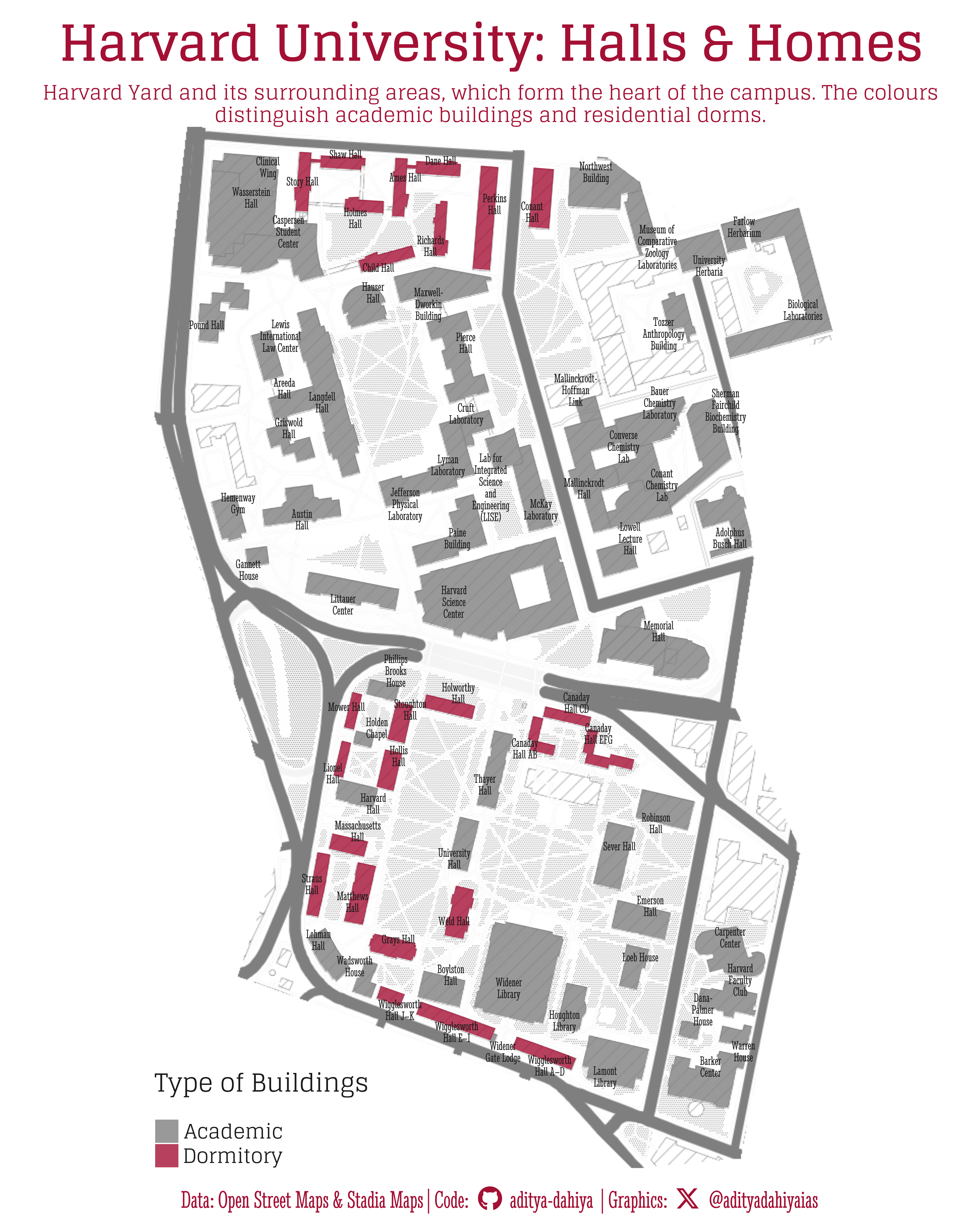
Figure 1: A detailed map of Harvard University’s campus, created using R and OpenStreetMap data. This visualization highlights key buildings, streets, and landmarks with custom styling for clarity and readability.

Loading required libraries, data import & creating custom functions.

# Data Wrangling & Plotting Tools
library(tidyverse)            # All things tidy
library(sf)                   # Simple Features in R

# Plot touch-up tools
library(scales)               # Nice Scales for ggplot2
library(fontawesome)          # Icons display in ggplot2
library(ggtext)               # Markdown text support for ggplot2
library(showtext)             # Display fonts in ggplot2
library(colorspace)           # Lighten and Darken colours


# Getting geographic data 
library(ggmap)                # Getting raster maps
library(terra)                # Cropping / Masking rasters
library(tidyterra)            # Rasters with ggplot2
library(osmdata)              # Open Street Maps data

Visualization Parameters

# Font for titles
font_add_google("Solway",
  family = "title_font"
) 

# Font for the caption
font_add_google("Stint Ultra Condensed",
  family = "caption_font"
) 

# Font for plot text
font_add_google("Glegoo",
  family = "body_font"
) 

showtext_auto()

mypal <- c("#A41034", "#68666F", "grey10", "white")


# A base Colour
bg_col <- mypal[4]
seecolor::print_color(bg_col)

# Colour for highlighted text
text_hil <- mypal[1]
seecolor::print_color(text_hil)

# Colour for the text
text_col <- mypal[3]
seecolor::print_color(text_col)


# Define Base Text Size
bts <- 90 

# Caption stuff for the plot
sysfonts::font_add(
  family = "Font Awesome 6 Brands",
  regular = here::here("docs", "Font Awesome 6 Brands-Regular-400.otf")
)
github <- "&#xf09b"
github_username <- "aditya-dahiya"
xtwitter <- "&#xe61b"
xtwitter_username <- "@adityadahiyaias"
social_caption_1 <- glue::glue("<span style='font-family:\"Font Awesome 6 Brands\";'>{github};</span> <span style='color: {text_hil}'>{github_username}  </span>")
social_caption_2 <- glue::glue("<span style='font-family:\"Font Awesome 6 Brands\";'>{xtwitter};</span> <span style='color: {text_hil}'>{xtwitter_username}</span>")
plot_caption <- paste0(
  "**Data:** Open Street Maps & Stadia Maps", 
  " |  **Code:** ", 
  social_caption_1, 
  " |  **Graphics:** ", 
  social_caption_2
  )
rm(github, github_username, xtwitter, 
   xtwitter_username, social_caption_1, 
   social_caption_2)

# Add text to plot-------------------------------------------------
plot_title <- "Harvard University: Halls & Homes"

plot_subtitle <- "Harvard Yard and its surrounding areas, which form the heart of the campus. The colours distinguish academic buildings and residential dorms."

Get custom data

# A custom boundary of Harvard Yard and surrounding areas
coords <- matrix(
  c(-71.11416707468163, 42.3720048391194,
    -71.11353806031005, 42.37440147585385,
    -71.1142580854591, 42.3755669937761,
    -71.11402806334283, 42.3766771432422,
    -71.11427340903329, 42.37819510823347,
    -71.11306194359479, 42.37841033600014,
    -71.11356707475474, 42.37950090804519,
    -71.11477964414628, 42.37936400535951,
    -71.11557374883363, 42.37980448108043,
    -71.1199935674755, 42.38004150690507,
    -71.12034348159067, 42.37780914536264,
    -71.11899327303243, 42.3744466643869,
    -71.11945738716973, 42.373425213014855,
    -71.11617254744829, 42.3725587572454,
    -71.11529708579101, 42.3719287901022,
    -71.11416707468163, 42.3720048391194), 
  byrow = TRUE, 
  ncol = 2
)

# Create an sf object
harvard_sf <- st_sf(
  geometry = st_sfc(st_polygon(list(coords))), 
  crs = "EPSG:4326"
  )
rm(coords)

harvard_buildings_raw <- opq(st_bbox(harvard_sf)) |> 
  add_osm_feature(
    key = "building",
    value = c("apartments", 
              "cathedral", "chapel", "church", 
              "college",
              "dormitory",
              "hotel", "house", 
              "library", 
              "museum", "office", 
              "residential", "school", "supermarket", 
               "train_station", "university"),
    key_exact = TRUE,
    value_exact = FALSE,
    match_case = FALSE
  ) |> 
  osmdata_sf()

harvard_buildings <- bind_rows(
  harvard_buildings_raw$osm_polygons,

  harvard_buildings_raw$osm_multipolygons
) |> 
  st_intersection(harvard_sf) |> 
  filter(!is.na(name)) |> 
  select(name, architect, building) |> 
  filter(building %in% c("dormitory", "university")) |> 
  mutate(
    building = case_when(
      name %in% c(
        "Conant Hall", "Child Hall", 
        "Richards Hall", "Perkins Hall", "Ames Hall",
        "Dane Hall", "Shaw Hall", "Holmes Hall", "Story Hall"
      ) ~ "dormitory",
      .default = building
    ),
    building = if_else(building == "university", "academic", building),
    building = str_to_title(building)
  )


# Making abounding box that Stadia Maps can understand
harvard_bbox <- sf::st_bbox(harvard_sf)

# A bounding box in the format c(lowerleftlon, lowerleftlat, upperrightlon, upperrightlat)
harvard_bbox <- c(
  left = harvard_bbox$xmin,
  right = harvard_bbox$xmax,
  bottom = harvard_bbox$ymin,
  top = harvard_bbox$ymax
)
names(harvard_bbox) <- c("left", "right", "bottom", "top")


# Register the Stadia Maps Key here
# register_stadiamaps("KEY")

raw_rast <- get_stadiamap(
  bbox = harvard_bbox,
  zoom = 17,
  maptype = "stamen_toner_background"
)

raw_rast2 <- get_stadiamap(
  bbox = harvard_bbox,
  zoom = 17,
  maptype = "stamen_watercolor"
)

rast1 <- rast(raw_rast) |> 
  crop(harvard_sf) |> 
  mask(harvard_sf)

rast2 <- rast(raw_rast2) |> 
  crop(harvard_sf) |> 
  mask(harvard_sf)

The Base Plot

g <- ggplot() +
  geom_spatraster_rgb(
    data = rast1,
    maxcell = Inf,
    alpha = 0.5
  ) +
  geom_sf(
    data = harvard_buildings,
    mapping = aes(fill = building),
    alpha = 0.8,
    colour = NA
  ) +
  scale_fill_manual(
    values = c("grey50", mypal[1])
  ) +
  ggrepel::geom_text_repel(
    data = harvard_buildings,
    mapping = aes(
      label = str_wrap(name, 10, whitespace_only = F),
      geometry = geometry
    ),
    family = "caption_font",
    colour = text_col,
    lineheight = 0.25,
    size = 16,
    stat = "sf_coordinates",
    min.segment.length = unit(50, "mm"),
    force_pull = 10
  ) +
  labs(
    title = plot_title,
    subtitle = str_wrap(plot_subtitle, 90),
    caption = plot_caption,
    fill = "Type of Buildings"
  ) +
  coord_sf(
    expand = FALSE,
    clip = "off"
  ) +
  ggthemes::theme_map(
    base_family = "body_font",
    base_size = bts
  ) +
  theme(
    
    # Full plot features
    plot.margin = margin(10,10,5,10, "mm"),
    plot.title.position = "plot",
    text = element_text(
      colour = text_col,
      margin = margin(0,0,0,0, "mm")
    ),
    
    # Legend
    legend.position = "inside",
    legend.position.inside = c(0,0),
    legend.justification = c(0,0),
    legend.margin = margin(0,0,0,0, "mm"),
    legend.box.margin = margin(0,0,0,0, "mm"),
    legend.text = element_text(
      margin = margin(0,0,0,2, "mm"),
      colour = text_col
    ),
    legend.title = element_text(
      margin = margin(0,0,10,0, "mm"),
      colour = text_col,
      hjust = 0,
      lineheight = 0.3
    ),
    legend.title.position = "top",
    legend.key.height = unit(10, "mm"),
    legend.key.width = unit(10, "mm"),
    legend.text.position = "right",
    
    # Labels and titles
    plot.title = element_text(
      hjust = 0.5,
      size = 2 * bts,
      lineheight = 0.3,
      margin = margin(0,0,5,0, "mm"),
      colour = text_hil,
      face = "bold"
    ),
    plot.subtitle = element_text(
      hjust = 0.5,
      size = 0.8 * bts,
      lineheight = 0.3,
      margin = margin(0,0,0,0, "mm"),
      colour = text_hil
    ),
    plot.caption = element_textbox(
      hjust = 0.5,
      family = "caption_font",
      lineheight = 0.3,
      margin = margin(0,0,0,0, "mm"),
      size = bts,
      colour = text_hil
    )
  )

ggsave(
  plot = g,
  filename = here::here(
    "data_vizs", "viz_harvard_yard1.png"
  ),
  height = 50,
  width = 40,
  units = "cm",
  bg = bg_col
)

Savings the thumbnail for the webpage

# Saving a thumbnail

library(magick)
# Saving a thumbnail for the webpage
image_read(here::here("data_vizs", 
                      "viz_harvard_yard1.png")) |> 
  image_resize(geometry = "x400") |> 
  image_write(
    here::here(
      "data_vizs", 
      "thumbnails", 
      "viz_harvard_yard.png"
    )
  )

Session Info

# Data Wrangling & Plotting Tools
library(tidyverse)            # All things tidy
library(sf)                   # Simple Features in R

# Plot touch-up tools
library(scales)               # Nice Scales for ggplot2
library(fontawesome)          # Icons display in ggplot2
library(ggtext)               # Markdown text support for ggplot2
library(showtext)             # Display fonts in ggplot2
library(colorspace)           # Lighten and Darken colours


# Getting geographic data 
library(ggmap)                # Getting raster maps
library(terra)                # Cropping / Masking rasters
library(tidyterra)            # Rasters with ggplot2
library(osmdata)              # Open Street Maps data

sessioninfo::session_info()$packages |> 
  as_tibble() |> 
  select(package, 
         version = loadedversion, 
         date, source) |> 
  arrange(package) |> 
  janitor::clean_names(
    case = "title"
  ) |> 
  gt::gt() |> 
  gt::opt_interactive(
    use_search = TRUE
  ) |> 
  gtExtras::gt_theme_espn()

Table 1: R Packages and their versions used in the creation of this page and graphics