Coal Clusters: Charting India’s Energy Sources

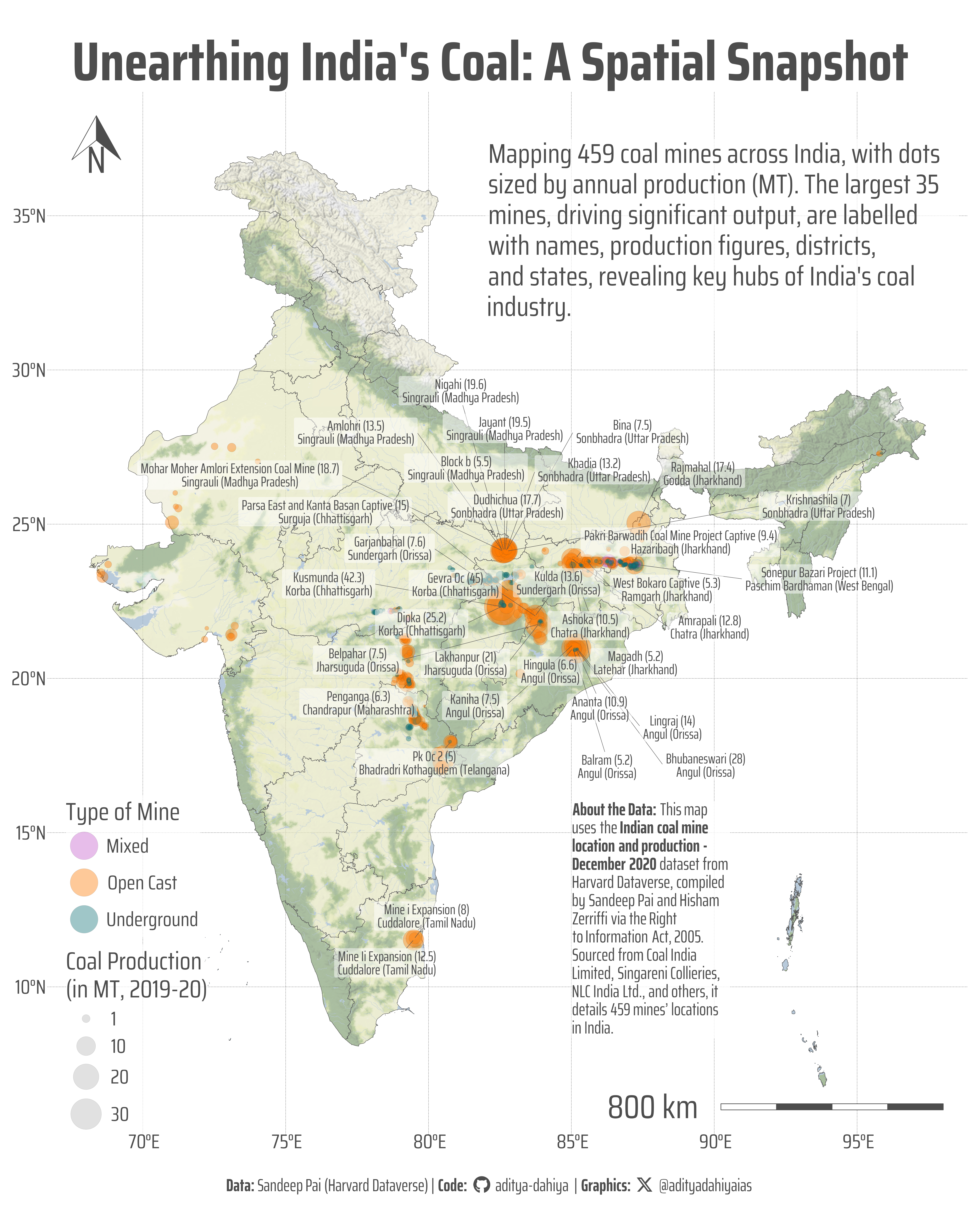
Mapping 459 coal mines across India, with dots sized by annual production (MT). The largest 35 mines, driving significant output, are labelled with names, production figures, districts, and states, revealing key hubs of India’s coal industry.

About the Data

The dataset, titled “Indian coal mine location and production - December 2020,” hosted on Harvard Dataverse, provides detailed information on coal mines in India, including geocoordinates and production data, ideal for mapping purposes. Compiled through applications under the Right to Information Act, 2005, it draws from major entities like Coal India Limited, Singareni Collieries Company Limited, NLC India Ltd., the Indian Coal Ministry, and the Coal Controller Organization. The data, initially in PDF format, was manually entered into Excel by the authors: Sandeep Pai and Hisham Zerriffi, with geocoordinates sourced from government documents or Google Maps. For further details, users can access the dataset at DOI:10.7910/DVN/TDEK8O.

Figure 1: This map visualizes 459 coal mines in India, with dots sized by annual production (MT). The largest 35 mines are labelled with names, output, districts, and states, highlighting key coal hubs. Data from Sandeep Pai and Hisham Zerriffi’s “Indian coal mine dataset.” Created using R packages: ggplot2, sf, tidyterra, ggmap, and ggrepel.

How I made this graphic?

The code generates a detailed map of coal mine locations in India using data from the “Indian coal mine location and production - December 2020” dataset, retrieved via the dataverse package. The Excel data is imported with readxl (alternatively, usign {dataverse} for directly getting the data from HArvard Dateverse, and cleaned using janitor. Geospatial data is processed with sf for vector layers and terra for raster data, integrated into ggplot2 visualizations via tidyterra. A base map is sourced using ggmap, with spatial enhancements like scales and north arrows added by ggspatial. Aesthetic improvements are made with scales, fontawesome, ggtext, showtext, and colorspace. Key techniques include geom_spatraster_rgb() for rendering the raster base map, geom_sf() for overlaying coal mine locations sized by production, and ggrepel::geom_label_repel() for non-overlapping labels of significant mines. The final plot is crafted and saved using ggplot2’s layering system, enhanced by custom fonts and themes.

Loading required libraries, data import

# Plot touch-up tools
library(scales)               # Nice Scales for ggplot2
library(fontawesome)          # Icons display in ggplot2
library(ggtext)               # Markdown text support for ggplot2
library(showtext)             # Display fonts in ggplot2
library(colorspace)           # Lighten and Darken colours


# Getting geographic data 
library(sf)                   # Simple Features in R
library(terra)                # Cropping / Masking rasters
library(tidyterra)            # Rasters with ggplot2
library(ggspatial)            # Scales and Arrows on maps

# Data Wrangling & ggplot2
library(tidyverse)            # All things tidy
library(patchwork)            # Composing plots

# Accessing Harvard Dataverse
library(dataverse)            # Access Harvard Dataverse

raw_data <- dataverse::get_dataframe_by_name(
  filename = "Indian Coal Mines Dataset_January 2021-1.tab",
  dataset = "doi:10.7910/DVN/TDEK8O",
  .f = readxl::read_excel,
  server = "dataverse.harvard.edu"
)

raw_data <- readxl::read_excel(
  path = "Indian Coal Mines Dataset_January 2021-1.xlsx",
  sheet = 2
) |> 
  janitor::clean_names()

Visualization Parameters

# Font for titles
font_add_google("Saira",
  family = "title_font"
) 

# Font for the caption
font_add_google("Saira Extra Condensed",
  family = "caption_font"
) 

# Font for plot text
font_add_google("Saira Condensed",
  family = "body_font"
) 

showtext_auto()
mypal <- c("#C35BCAFF", "#FD7901FF", "#0E7175FF")

# A base Colour
bg_col <- "white"
seecolor::print_color(bg_col)

# Colour for highlighted text
text_hil <- "grey30"
seecolor::print_color(text_hil)

# Colour for the text
text_col <- "grey20"
seecolor::print_color(text_col)

# Define Base Text Size
bts <- 90 

# Caption stuff for the plot
sysfonts::font_add(
  family = "Font Awesome 6 Brands",
  regular = here::here("docs", "Font Awesome 6 Brands-Regular-400.otf")
)
github <- "&#xf09b"
github_username <- "aditya-dahiya"
xtwitter <- "&#xe61b"
xtwitter_username <- "@adityadahiyaias"
social_caption_1 <- glue::glue("<span style='font-family:\"Font Awesome 6 Brands\";'>{github};</span> <span style='color: {text_hil}'>{github_username}  </span>")
social_caption_2 <- glue::glue("<span style='font-family:\"Font Awesome 6 Brands\";'>{xtwitter};</span> <span style='color: {text_hil}'>{xtwitter_username}</span>")
plot_caption <- paste0(
  "**Data:** Sandeep Pai (Harvard Dataverse)", 
  " |  **Code:** ", 
  social_caption_1, 
  " |  **Graphics:** ", 
  social_caption_2
  )
rm(github, github_username, xtwitter, 
   xtwitter_username, social_caption_1, 
   social_caption_2)

# Alpha Values for dots and colours
alpha_value = 0.6

# Add text to plot-------------------------------------------------
plot_title <- "Unearthing India's Coal: A Spatial Snapshot"

plot_subtitle <- "Mapping 459 coal mines across India, with dots sized by annual production (MT). The largest 35 mines, driving significant output, are labelled with names, production figures, districts, and states, revealing key hubs of India's coal industry."

data_annotation <- "**About the Data:** This map uses the **Indian coal mine location and production - December 2020** dataset from Harvard Dataverse, compiled by Sandeep Pai and Hisham Zerriffi via the *Right to Information Act, 2005*. Sourced from Coal India Limited, Singareni Collieries, NLC India Ltd., and others, it details *459 mines' locations* in India." |> 
  str_wrap(30) |> 
  str_replace_all("\\n", "<br>")

Data Wrangling

# Background Raster Map
library(ggmap)

bbox_raster <- india_map |> 
  st_bbox()
names(bbox_raster) <- c("left", "bottom", "right", "top")  
base_raster_raw <- get_stadiamap(
  bbox = bbox_raster,
  zoom = 7,
  maptype = "stamen_terrain_background"
)
rast_crs <- rast(base_raster_raw) |> crs()

base_raster <- rast(base_raster_raw) |>
  terra::crop(india_map) |> 
  terra::mask(india_map)


# Vector Map of India
india_map <- read_sf(
  here::here(
    "data", "india_map", 
    "India_State_Boundary.shp"
  )
) |> 
  st_transform("EPSG:4326") |> 
  st_transform(rast_crs)

# raw_data |> 
#   dplyr::distinct(type_of_mine_oc_ug_mixed)
# 
# raw_data |> names()

df1 <- raw_data |> 
  mutate(
    mine_name = snakecase::to_title_case(mine_name),
    type_of_mine = case_when(
      type_of_mine_oc_ug_mixed == "UG" ~ "Underground",
      type_of_mine_oc_ug_mixed == "OC" ~ "Open Cast",
      type_of_mine_oc_ug_mixed == "Mixed" ~ "Mixed"
    )
  ) |> 
  rename(
    production = coal_lignite_production_mt_2019_2020,
    mine_type = type_of_mine
  ) |> 
  select(
    state_ut_name, district_name, mine_name,
    production, mine_type,
    coal_mine_owner_name,
    latitude, longitude
  ) |> 
  arrange(desc(production)) |> 
  st_as_sf(coords = c("longitude", "latitude")) |> 
  st_set_crs("EPSG:4326") |> 
  st_transform(rast_crs)
  
# df1 |> 
#   st_drop_geometry() |> 
#   ggplot() +
#   geom_boxplot(aes(production))
# 
# df1 |> 
#   filter(production > 5)

# ggplot() +
#   geom_spatraster_rgb(
#     data = base_raster,
#     alpha = alpha_value
#   )

df1 |> 
  st_drop_geometry() |> 
  filter(production > 5)

Composing Final Plot

g <- ggplot() +
  geom_spatraster_rgb(
    data = base_raster,
    alpha = 0.7,
    maxcell = Inf
  ) +
  geom_sf(
    data = india_map,
    fill = NA
  ) +
  geom_sf(
    data = df1,
    mapping = aes(
      size = production,
      fill = mine_type
    ),
    alpha = 0.4,
    pch = 21,
    stroke = 0.1,
    colour = text_col
  ) |> ggblend::blend("darken") +
  scale_size_continuous(
    range = c(1.5, 20),
    breaks = c(1, 10, 20, 30)
  ) +
  scale_fill_manual(
    values = mypal
  ) +
  ggrepel::geom_label_repel(
    data = df1 |> filter(production > 5),
    mapping = aes(
      geometry = geometry,
      label = paste0(mine_name, " (", 
                     round(production, 1), ")\n",
                     district_name, " (", state_ut_name,")"
                     )
    ),
    family = "caption_font",
    segment.size = 0.2,
    min.segment.length = unit(0.1, "pt"),
    force = 10,
    force_pull = 0.001,
    stat = "sf_coordinates",
    lineheight = 0.25,
    size = bts / 5,
    max.overlaps = 40,
    fill = alpha(bg_col, 0.5),
    label.size = NA,
    colour = text_hil
  ) +
  
  # Add Plot subtitle
  annotate(
    geom = "label",
    x = 82,
    y = 37.5,
    label = str_wrap(plot_subtitle, 50),
    size = bts / 2.6,
    lineheight = 0.3,
    hjust = 0,
    vjust = 1,
    family = "body_font",
    fill = alpha(bg_col, 0.7),
    label.size = NA,
    label.padding = unit(0.1, "lines"),
    colour = text_hil
  ) +
  # Add annotation on about the data
  annotate(
    geom = "richtext",
    x = 85,
    y = 16,
    label = data_annotation,
    size = bts / 4,
    lineheight = 0.33,
    hjust = 0,
    vjust = 1,
    family = "caption_font",
    fill = alpha(bg_col, 0.8),
    label.size = NA,
    label.padding = unit(0.1, "lines"),
    colour = text_hil
  ) +
  
  # Add Map annotations
  ggspatial::annotation_north_arrow(
    location = "tl",
    height = unit(2, "cm"),
    width = unit(2, "cm"),
    style = ggspatial::north_arrow_orienteering(
      line_col = text_hil,
      text_col = text_hil,
      text_family = "body_font",
      fill = c(bg_col, text_hil),
      text_size = bts * 1.5
    ),
    pad_x = unit(1, "cm"),
    pad_y = unit(1, "cm"),
    text_pad = unit(1, "cm")
  ) +
  ggspatial::annotation_scale(
    location = "br",
    bar_cols = c(bg_col, text_hil),
    text_family = "body_font",
    text_cex = bts / 9,
    text_col = text_hil,
    line_col = text_hil,
    pad_x = unit(1, "cm"),
    pad_y = unit(1, "cm"),
    text_pad = unit(1, "cm")
  ) +
  
  # Legends and Labels
  labs(
    title = plot_title,
    caption = plot_caption,
    size = "Coal Production\n(in MT, 2019-20)",
    fill = "Type of Mine",
    x = NULL, y = NULL
  ) +
  guides(
    fill = guide_legend(
      override.aes = list(
        size = 15, pch = 21
      )
    ),
    size = guide_legend(
      override.aes = list(
        pch = 21,
        colour = text_col,
        fill = "grey70"
      )
    )
  ) +
  
  # Theme and beautification of plot
  theme_minimal(
    base_family = "body_font",
    base_size = bts
  ) +
  theme(
    
    # Overall
    plot.margin = margin(5,5,5,5, "mm"),
    plot.title.position = "plot",
    plot.caption.position = "plot",
    text = element_text(
        colour = text_hil
    ), 
    
    # Grid and Axes
    panel.grid = element_line(
      linewidth = 0.2,
      colour = text_hil,
      linetype = 3
    ),
    axis.text.x = element_text(margin = margin(0,0,0,0, "mm")),
    axis.text.y = element_text(margin = margin(0,0,0,0, "mm")),
    axis.ticks = element_blank(),
    axis.ticks.length = unit(0, "mm"),
    
    # Legend
    legend.position = "inside",
    legend.position.inside = c(0.02, 0),
    legend.justification = c(0, 0),
    legend.title.position = "top",
    legend.direction = "vertical",
    legend.box = "vertical",
    legend.title = element_text(
      margin = margin(2,0,2,0, "mm"),
      hjust = 0,
      lineheight = 0.3
    ),
    legend.text = element_text(
      margin = margin(2,0,2,2, "mm"),
      hjust = 0
    ),
    legend.text.position = "right",
    legend.background = element_rect(
      fill = alpha("white", 0.7), colour = NA
    ),
    legend.margin = margin(0,0,0,0, "mm"),
    legend.box.margin = margin(0,0,0,0, "mm"),
    legend.spacing.y = unit(3, "mm"),
    legend.spacing.x = unit(1, "mm"),
    
    # Labels
    plot.title = element_text(
      hjust = 0.5,
      size = bts * 2.2,
      margin = margin(5,0,0,0, "mm"),
      family = "body_font",
      lineheight = 0.3,
      face = "bold"
    ),
    plot.subtitle = element_text(
      hjust = 0.5, 
      family = "body_font",
      lineheight = 0.3,
      margin = margin(0,0,0,0, "mm")
    ),
    plot.caption = element_textbox(
      hjust = 0.5,
      halign = 0.5, 
      margin = margin(10,0,0,0, "mm"),
      family = "caption_font",
      size = 0.7 * bts
    )
  )


ggsave(
  plot = g,
  filename = here::here(
    "data_vizs", "viz_india_coalmines.png"
  ),
  height = 50,
  width = 40,
  units = "cm",
  bg = bg_col
)  

Savings the thumbnail for the webpage

# Saving a thumbnail

library(magick)
# Saving a thumbnail for the webpage
image_read(here::here("data_vizs", 
                      "viz_india_coalmines.png")) |> 
  image_resize(geometry = "x400") |> 
  image_write(
    here::here(
      "data_vizs", 
      "thumbnails", 
      "viz_india_coalmines.png"
    )
  )

Session Info

# Plot touch-up tools
library(scales)               # Nice Scales for ggplot2
library(fontawesome)          # Icons display in ggplot2
library(ggtext)               # Markdown text support for ggplot2
library(showtext)             # Display fonts in ggplot2
library(colorspace)           # Lighten and Darken colours


# Getting geographic data 
library(sf)                   # Simple Features in R
library(terra)                # Cropping / Masking rasters
library(tidyterra)            # Rasters with ggplot2
library(ggspatial)            # Scales and Arrows on maps

# Data Wrangling & ggplot2
library(tidyverse)            # All things tidy
library(patchwork)            # Composing plots

# Accessing Harvard Dataverse
library(dataverse)            # Access Harvard Dataverse

sessioninfo::session_info()$packages |> 
  as_tibble() |> 
  select(package, 
         version = loadedversion, 
         date, source) |> 
  arrange(package) |> 
  janitor::clean_names(
    case = "title"
  ) |> 
  gt::gt() |> 
  gt::opt_interactive(
    use_search = TRUE
  ) |> 
  gtExtras::gt_theme_espn()

Table 1: R Packages and their versions used in the creation of this page and graphics