Exploring London’s Rivers & Bridges

This map visualizes London’s rivers and bridges using OpenStreetMap data, processed with R’s sf, osmdata, and terra packages. A smooth basemap, automated labeling, and refined aesthetics enhance clarity and readability.

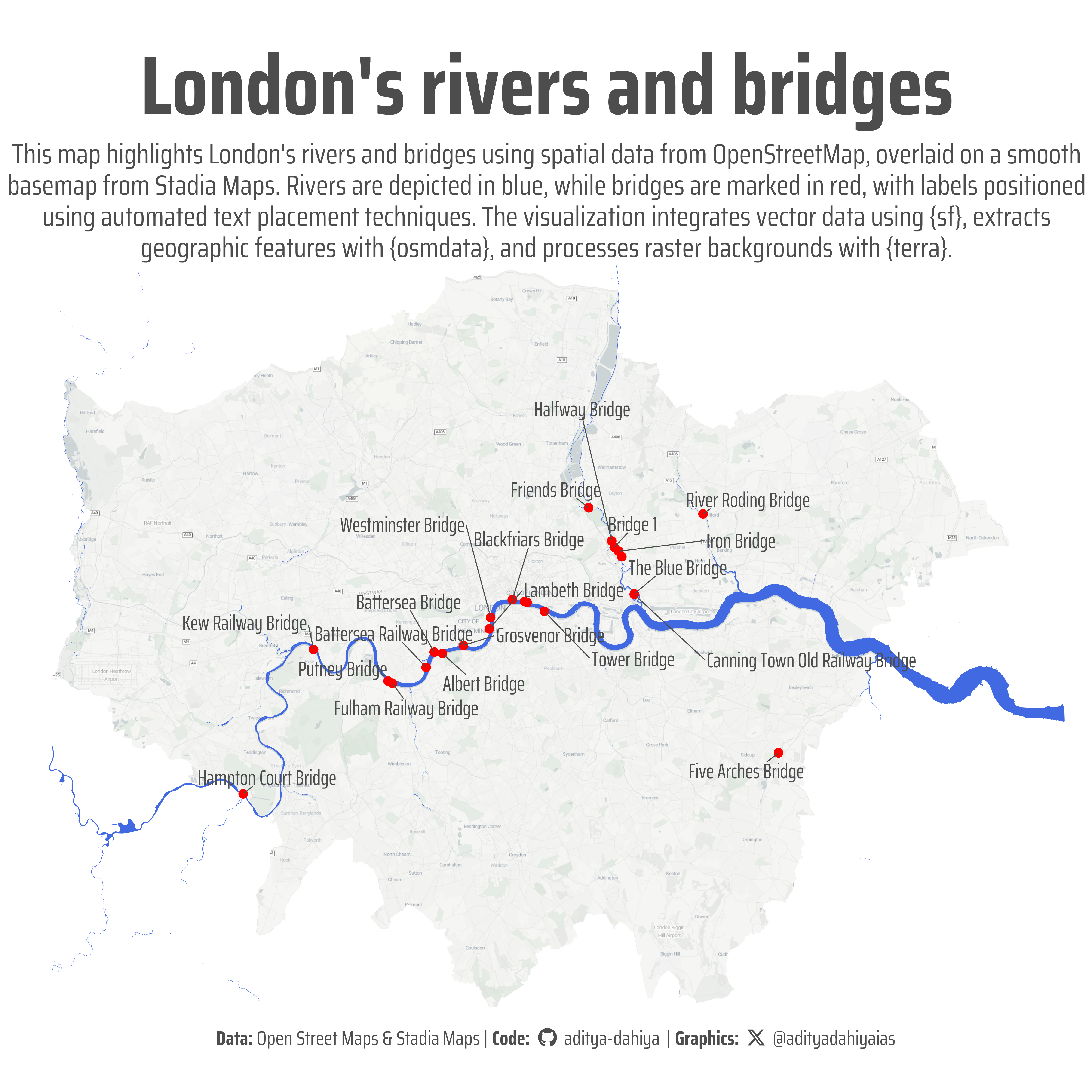
This visualization maps London’s rivers and bridges using spatial data from OpenStreetMap and background tiles from Stadia Maps. The analysis leverages sf for spatial operations, osmdata for extracting waterways and bridges, and terra for raster processing. The plot integrates a semi-transparent base map with rivers in blue and bridges in red. Labels are placed using ggrepel, and the final design is enhanced with ggtext and showtext. The result is a detailed yet aesthetic map, exported as a high-resolution PNG.

Figure 1: This map showcases London’s rivers and bridges, extracted from OpenStreetMap and overlaid on a smooth basemap. Rivers are highlighted in blue, while bridges are marked in red, with automated labels for clarity. The visualization combines spatial data processing with refined aesthetics to create an informative and visually appealing representation.

Loading required libraries, data import & creating custom functions.

# Data Wrangling & Plotting Tools
library(tidyverse)            # All things tidy
library(sf)                   # Simple Features in R

# Plot touch-up tools
library(scales)               # Nice Scales for ggplot2
library(fontawesome)          # Icons display in ggplot2
library(ggtext)               # Markdown text support for ggplot2
library(showtext)             # Display fonts in ggplot2
library(colorspace)           # Lighten and Darken colours


# Getting geographic data 
library(ggmap)                # Getting raster maps
library(terra)                # Cropping / Masking rasters
library(tidyterra)            # Rasters with ggplot2
library(osmdata)              # Open Street Maps data

Visualization Parameters

# Font for titles
font_add_google("Saira",
  family = "title_font"
) 

# Font for the caption
font_add_google("Saira Extra Condensed",
  family = "caption_font"
) 

# Font for plot text
font_add_google("Saira Condensed",
  family = "body_font"
) 

showtext_auto()

mypal <- c("red", "royalblue", "grey30", "grey10")

# A base Colour
bg_col <- "white"
seecolor::print_color(bg_col)

# Colour for highlighted text
text_hil <- mypal[3]
seecolor::print_color(text_hil)

# Colour for the text
text_col <- mypal[3]
seecolor::print_color(text_col)


# Define Base Text Size
bts <- 90 

# Caption stuff for the plot
sysfonts::font_add(
  family = "Font Awesome 6 Brands",
  regular = here::here("docs", "Font Awesome 6 Brands-Regular-400.otf")
)
github <- "&#xf09b"
github_username <- "aditya-dahiya"
xtwitter <- "&#xe61b"
xtwitter_username <- "@adityadahiyaias"
social_caption_1 <- glue::glue("<span style='font-family:\"Font Awesome 6 Brands\";'>{github};</span> <span style='color: {text_hil}'>{github_username}  </span>")
social_caption_2 <- glue::glue("<span style='font-family:\"Font Awesome 6 Brands\";'>{xtwitter};</span> <span style='color: {text_hil}'>{xtwitter_username}</span>")
plot_caption <- paste0(
  "**Data:** Open Street Maps & Stadia Maps", 
  " |  **Code:** ", 
  social_caption_1, 
  " |  **Graphics:** ", 
  social_caption_2
  )
rm(github, github_username, xtwitter, 
   xtwitter_username, social_caption_1, 
   social_caption_2)

# Add text to plot-------------------------------------------------
plot_title <- "London's rivers and bridges"

plot_subtitle <- "This map highlights London's rivers and bridges using spatial data from OpenStreetMap, overlaid on a smooth basemap from Stadia Maps. Rivers are depicted in blue, while bridges are marked in red, with labels positioned using automated text placement techniques. The visualization integrates vector data using {sf}, extracts geographic features with {osmdata}, and processes raster backgrounds with {terra}."

Get custom data

london_city_sf <- spData::lnd |> 
  janitor::clean_names() |> 
  select(name, geometry)

london_city_boundary <- london_city_sf |> 
  st_union()

# ggplot(london_city_boundary) +
#   geom_sf()


london_rivers <- opq(st_bbox(london_city_boundary)) |> 
  add_osm_feature(
    key = "water",
    value = c("river"),
    key_exact = TRUE,
    value_exact = FALSE,
    match_case = FALSE
  ) |> 
  osmdata_sf()

london_bridges <- opq(st_bbox(london_city_boundary)) |> 
  add_osm_features(
    features = list(
      "man_made" = "bridge",
      "building" = "bridge"
    ),
    key_exact = TRUE,
    value_exact = FALSE
  ) |> 
  osmdata_sf()

df_rivers <- bind_rows(
  london_rivers$osm_multipolygons |> 
    select(name),
  london_rivers$osm_polygons |> 
    select(name),
  london_rivers$osm_lines |> 
    select(name)
)

df_bridges <- bind_rows(
  london_bridges$osm_points |> 
    select(name),
  london_bridges$osm_lines |> 
    select(name),
  london_bridges$osm_polygons |> 
    select(name),
  london_bridges$osm_multipolygons |> 
    select(name),
  london_bridges$osm_multilines |> 
    select(name)
) |> 
  st_cast("POINT") |> 
  filter(!is.na(name)) |> 
  st_intersection(london_city_boundary)

nearby_bridges <- df_bridges |> 
  st_is_within_distance(df_rivers, dist = 10, sparse = TRUE)

df_bridges <- df_bridges[lengths(nearby_bridges) > 0, ]

# Making abounding box that Stadia Maps can understand
london_bbox <- sf::st_bbox(london_city_boundary)

# A bounding box in the format c(lowerleftlon, lowerleftlat, upperrightlon, upperrightlat)
london_bbox <- c(
  left = london_bbox$xmin,
  right = london_bbox$xmax,
  bottom = london_bbox$ymin,
  top = london_bbox$ymax
)
names(london_bbox) <- c("left", "right", "bottom", "top")


# Register the Stadia Maps Key here
# register_stadiamaps("KEY")
raw_rast <- get_stadiamap(
  bbox = london_bbox,
  zoom = 12,
  maptype = "alidade_smooth"
)

rast1 <- rast(raw_rast) |> 
  crop(london_city_sf) |> 
  mask(london_city_sf)

The Base Plot

g <- ggplot() +
  geom_spatraster_rgb(
    data = rast1,
    alpha = 0.8,
    maxcell = Inf
  ) +
  geom_sf(
    data = df_rivers,
    fill = mypal[2],
    colour = "transparent"
  ) + 
  geom_sf(
    data = df_bridges,
    colour = mypal[1],
    size = 4
  ) +
  ggrepel::geom_text_repel(
    data = df_bridges,
    mapping = aes(
      label = name,
      geometry = geometry
    ),
    family = "caption_font",
    colour = text_col,
    lineheight = 0.25,
    size = 24,
    stat = "sf_coordinates",
    min.segment.length = unit(2, "mm"),
    force = 30,
    force_pull = 0.0001
  ) +
  labs(
    title = plot_title,
    subtitle = str_wrap(plot_subtitle, 110),
    caption = plot_caption
  ) +
  coord_sf(
    expand = FALSE,
    clip = "off"
  ) +
  ggthemes::theme_map(
    base_family = "body_font",
    base_size = bts
  ) +
  theme(
    
    # Full plot features
    plot.margin = margin(10,10,5,10, "mm"),
    plot.title.position = "plot",
    text = element_text(
      colour = text_col,
      margin = margin(0,0,0,0, "mm")
    ),
    
    # Labels and titles
    plot.title = element_text(
      hjust = 0.5,
      size = 3 * bts,
      lineheight = 0.3,
      margin = margin(0,0,5,0, "mm"),
      colour = text_hil,
      face = "bold"
    ),
    plot.subtitle = element_text(
      hjust = 0.5,
      size = bts,
      lineheight = 0.3,
      margin = margin(0,0,0,0, "mm"),
      colour = text_hil
    ),
    plot.caption = element_textbox(
      hjust = 0.5,
      family = "body_font",
      lineheight = 0.3,
      margin = margin(0,0,0,0, "mm"),
      size = 0.7 * bts,
      colour = text_hil
    )
  )

ggsave(
  plot = g,
  filename = here::here(
    "data_vizs", "viz_london_bridges.png"
  ),
  height = 40,
  width = 40,
  units = "cm",
  bg = bg_col
)

Savings the thumbnail for the webpage

# Saving a thumbnail

library(magick)
# Saving a thumbnail for the webpage
image_read(here::here("data_vizs", 
                      "viz_london_bridges.png")) |> 
  image_resize(geometry = "x400") |> 
  image_write(
    here::here(
      "data_vizs", 
      "thumbnails", 
      "viz_london_bridges.png"
    )
  )

Session Info

# Data Wrangling & Plotting Tools
library(tidyverse)            # All things tidy
library(sf)                   # Simple Features in R

# Plot touch-up tools
library(scales)               # Nice Scales for ggplot2
library(fontawesome)          # Icons display in ggplot2
library(ggtext)               # Markdown text support for ggplot2
library(showtext)             # Display fonts in ggplot2
library(colorspace)           # Lighten and Darken colours


# Getting geographic data 
library(ggmap)                # Getting raster maps
library(terra)                # Cropping / Masking rasters
library(tidyterra)            # Rasters with ggplot2
library(osmdata)              # Open Street Maps data

sessioninfo::session_info()$packages |> 
  as_tibble() |> 
  select(package, 
         version = loadedversion, 
         date, source) |> 
  arrange(package) |> 
  janitor::clean_names(
    case = "title"
  ) |> 
  gt::gt() |> 
  gt::opt_interactive(
    use_search = TRUE
  ) |> 
  gtExtras::gt_theme_espn()

Table 1: R Packages and their versions used in the creation of this page and graphics