Guardians of the Keys: The Electors of the Next Pope

This graphic was created in R using a combination of web scraping, image processing, and data visualization techniques. It combines the power of rvest, magick, and ggplot2—along with geom_image and custom grid layouts—to transform structured Vatican data into a clear, visual story of papal influence.

Who Will Choose the Next Pope?

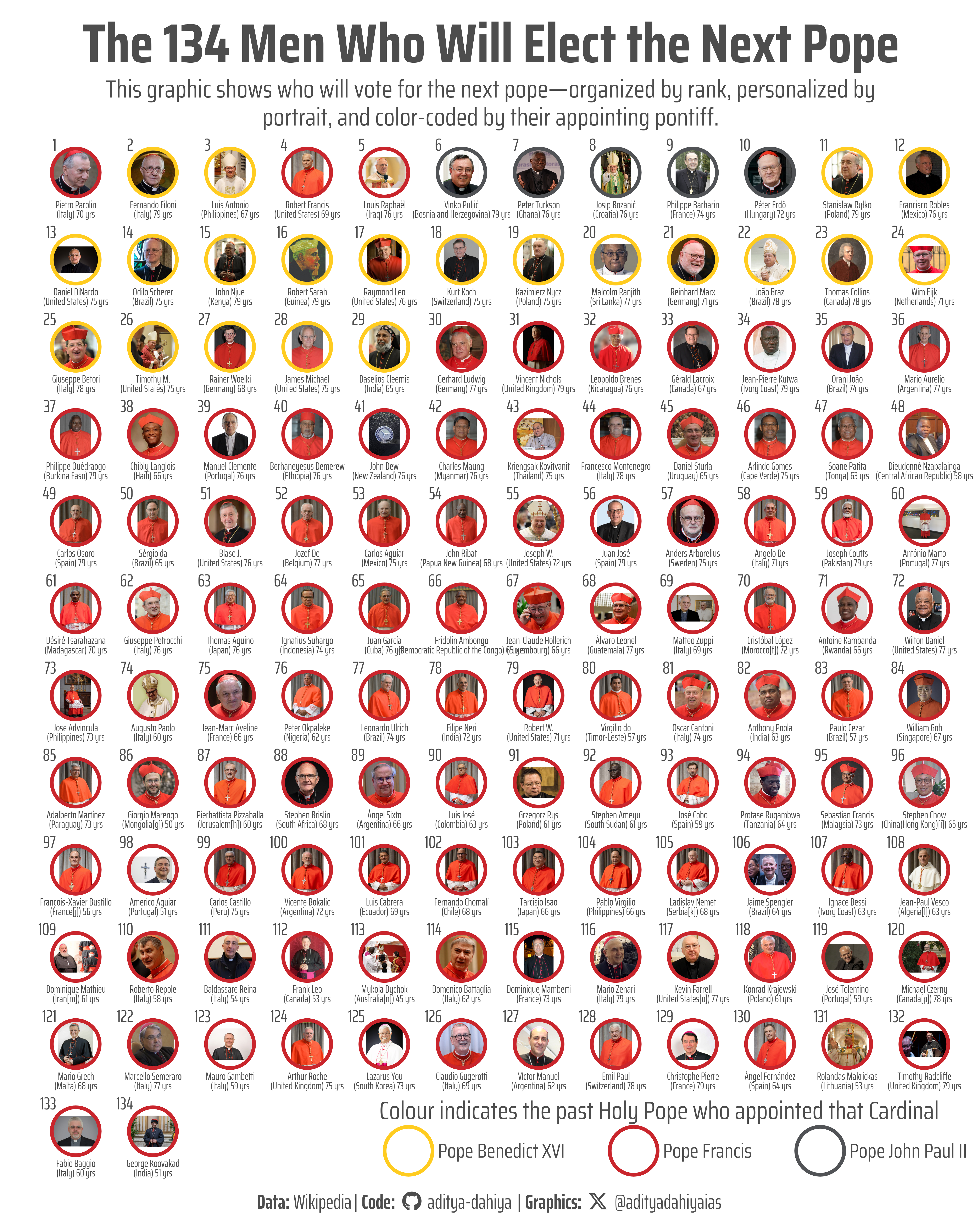
This grid visualization shows the 134 cardinal electors eligible to vote in the next papal conclave. Each circle represents a cardinal, arranged by their ecclesiastical rank (Cardinal-Bishop, -Priest, -Deacon), with portrait images cropped uniformly. The color of each circle’s border indicates which pope appointed them: St. John Paul II, Pope Benedict XVI, and Pope Francis.

What stands out is the overwhelming number of electors—over 70%—appointed by Pope Francis. This dramatic shift means the next pope is likely to reflect his theological priorities and pastoral tone. The graphic offers a clear visual narrative of influence and succession, making it easier to grasp how Church leadership has evolved over the past three decades.

This isn’t just a chart of faces—it’s a window into how the future of the Catholic Church is being shaped today.

Figure 1: Portraits of the 134 cardinal electors who will vote in the next papal conclave, arranged by ecclesiastical rank. Circle border colors indicate the pope who appointed each cardinal.

About the Data

The data for this visualization originates from the Wikipedia article Cardinal electors in the 2025 papal conclave, which provides a comprehensive and up-to-date list of the 135 cardinal electors eligible to participate in the upcoming conclave following the death of Pope Francis on April 21, 2025. This resource compiles information from official Vatican sources, including the Holy See Press Office and the Annuarium Statisticum Ecclesiae, and details each cardinal’s name, country, date of birth, ecclesiastical order (bishop, priest, or deacon), date of appointment (consistory), and the pope who appointed them. Notably, it also tracks changes in eligibility, such as Cardinal Antonio Cañizares Llovera’s decision not to attend due to health reasons, reducing the number of expected participants to 134. The dataset reflects the global composition of the College of Cardinals, with representation from 71 countries across six continents, and highlights that Pope Francis appointed 108 of the 135 electors, underscoring his significant influence on the Church’s future leadership. (Cardinal electors in the 2025 papal conclave)

How I made this graphic?

To create this visualization, I first collected the list of cardinal electors from Wikipedia and scraped their portraits using the rvest package in R. Each image was then processed and uniformly cropped using the magick package and cropcircles package to focus on faces. I categorized the cardinals by rank and identified the pope who appointed each using available Vatican sources. For plotting, I used ggplot2 with a custom grid layout inspired by the geom_image() and geom_point() to overlay portraits inside colored borders.

Loading required libraries

pacman::p_load(
  tidyverse,            # All things tidy
  
  scales,               # Nice Scales for ggplot2
  fontawesome,          # Icons display in ggplot2
  ggtext,               # Markdown text support for ggplot2
  showtext,             # Display fonts in ggplot2
  colorspace,           # Lighten and Darken colours
  
  magick,               # Download images and edit them
  ggimage,              # Display images in ggplot2
  patchwork,            # Composing Plots
  rvest                 # Web-Scraping
)

# URL of the Wikipedia page
# Read the HTML content of the page
page <- read_html("https://en.wikipedia.org/wiki/Cardinal_electors_in_the_2025_papal_conclave")

# Extract the first table (which contains the list of cardinals)
table_df <- page |> 
  html_table(fill = TRUE)
table_df <- table_df[[1]]

# Ensure the table is a tibble
cardinals <- as_tibble(table_df) |> 
  janitor::clean_names() |> 
  mutate(
    # Extract the date string from raw data
    born = str_extract(born, "^\\d{1,2} \\w+ \\d{4}"),
    # Convert to Date format
    born = dmy(born),  
    
    # Calculate age for each cardinal in years
    age = time_length(
      interval(
        start = born, 
        end = today()), 
        unit = "years") |> 
      floor()

  ) |> 
  mutate(
    date_consistory = str_extract(
      consistory, "^\\d{1,2} \\w+ \\d{4}"
      ) |>  dmy(),
    pope_consistory = str_remove(
      consistory, "^\\d{1,2} \\w+ \\d{4}"
      ) |>  str_trim(),
    pope_consistory = paste0("Pope ", pope_consistory),
    .keep = "unused"
  ) |> 
  select(-ref)

rm(page, table_df)

Visualization Parameters

# Font for titles
font_add_google("Saira",
  family = "title_font"
) 

# Font for the caption
font_add_google("Saira Extra Condensed",
  family = "caption_font"
) 

# Font for plot text
font_add_google("Saira Condensed",
  family = "body_font"
) 

showtext_auto()

# cols4all::c4a_gui()

mypal <- c("#FFCC20", "#C9252C", "#515356")

# A base Colour
bg_col <- "white"
seecolor::print_color(bg_col)

# Colour for highlighted text
text_hil <- "grey30"
seecolor::print_color(text_hil)

# Colour for the text
text_col <- "grey30"
seecolor::print_color(text_col)

line_col <- "grey30"

# Define Base Text Size
bts <- 90

# Caption stuff for the plot
sysfonts::font_add(
  family = "Font Awesome 6 Brands",
  regular = here::here("docs", "Font Awesome 6 Brands-Regular-400.otf")
)
github <- "&#xf09b"
github_username <- "aditya-dahiya"
xtwitter <- "&#xe61b"
xtwitter_username <- "@adityadahiyaias"
social_caption_1 <- glue::glue("<span style='font-family:\"Font Awesome 6 Brands\";'>{github};</span> <span style='color: {text_hil}'>{github_username}  </span>")
social_caption_2 <- glue::glue("<span style='font-family:\"Font Awesome 6 Brands\";'>{xtwitter};</span> <span style='color: {text_hil}'>{xtwitter_username}</span>")
plot_caption <- paste0(
  "**Data:** Wikipedia", 
  " |  **Code:** ", 
  social_caption_1, 
  " |  **Graphics:** ", 
  social_caption_2
  )
rm(github, github_username, xtwitter, 
   xtwitter_username, social_caption_1, 
   social_caption_2)

# Add text to plot-------------------------------------------------
plot_title <- "The 134 Men Who Will Elect the Next Pope"

plot_subtitle <- "This graphic shows who will vote for the next pope—organized by rank, personalized by portrait, and color-coded by their appointing pontiff."

Get temporary files on images of each Cardinal

# Get a custom google search engine and API key
# Tutorial: https://developers.google.com/custom-search/v1/overview
# Tutorial 2: https://programmablesearchengine.google.com/

# From:https://developers.google.com/custom-search/v1/overview
# google_api_key <- "LOAD YOUR GOOGLE API KEY HERE"

# From: https://programmablesearchengine.google.com/controlpanel/all
# my_cx <- "GET YOUR CUSTOM SEARCH ENGINE ID HERE"

# Improved function to download and save food images
download_cardinal_potrait <- function(i) {
  
  api_key <- google_api_key
  cx <- my_cx
  
  # Build the API request URL with additional filters
  url <- paste0(
    "https://www.googleapis.com/customsearch/v1?q=",
    URLencode(paste0("Cardinal ", cardinals$name[i], 
                     " photo potrait")),
    "&cx=", cx,
    "&searchType=image",
    "&key=", api_key,
    # "&imgSize=large",       # Restrict to medium-sized images
    # "&imgType=photo",
    "&num=1"                 # Fetch only one result
  )
  
  # Make the request
  response <- httr::GET(url)
  if (response$status_code != 200) {
    warning("Failed to fetch data for Cardinal: ", 
            cardinals$name[i])
    return(NULL)
  }
  
  # Parse the response
  result <- httr::content(response, "parsed")
  
  # Extract the image URL
  if (!is.null(result$items)) {
    image_url <- result$items[[1]]$link
  } else {
    warning("No results found for Cardinal: ", cardinals$name[i])
    return(NULL)
  }
  
  # Process the image
  im <- magick::image_read(image_url) |> 
      image_resize("x300") 
  
  # Calculate the new dimension for the square
  max_dim <- max(image_info(im)$width, image_info(im)$height)
  
  # Create a blank white canvas of square size
  canvas <- image_blank(width = max_dim, 
                        height = max_dim, 
                        color = bg_col)
  
  # Composite the original image onto the center of the square canvas
  image_composite(canvas, im, gravity = "center") |> 
    # Crop the image into a circle 
    # (Credits: https://github.com/doehm/cropcircles)
    cropcircles::circle_crop(
      border_colour = text_col,
      border_size = 2
    ) |>
    image_read() |> 
    image_background(color = bg_col) |> 
    image_resize("x300") |> 
    # Save or display the result
    image_write(
      here::here(
        "data_vizs", 
        paste0("temp_cardinals_", i, ".png")
        )
    )
}

# Iterate and download images
for (i in 132:nrow(cardinals)) {
  download_cardinal_potrait(i)
}

# MANUAALY NOTE DOWN
# Problematic indices - values for i for which the api did not work
problem_numbers <- c(
  7, 8, 15, 26, 27, 51, 76, 84, 95, 101,
  103, 104, 105, 112, 118, 131
  )

For some Cardinals, change the text of the query to get it successfully through API

# Improved function to download and save food images
download_cardinal_potrait_2 <- function(i) {
  
  api_key <- google_api_key
  cx <- my_cx
  
  # Build the API request URL with additional filters
  url <- paste0(
    "https://www.googleapis.com/customsearch/v1?q=",
    URLencode(paste0("Cardinal ", cardinals$name[i], 
                     " photo")),
    "&cx=", cx,
    "&searchType=image",
    "&key=", api_key
  )
  
  # Make the request
  response <- httr::GET(url)
  if (response$status_code != 200) {
    warning("Failed to fetch data for Cardinal: ", 
            cardinals$name[i])
    return(NULL)
  }
  
  # Parse the response
  result <- httr::content(response, "parsed")
  
  # Extract the image URL
  if (!is.null(result$items)) {
    image_url <- result$items[[1]]$link
  } else {
    warning("No results found for Cardinal: ", cardinals$name[i])
    return(NULL)
  }
  
  # Process the image
  im <- magick::image_read(image_url) |> 
      image_resize("x300") 
  
  # Calculate the new dimension for the square
  max_dim <- max(image_info(im)$width, image_info(im)$height)
  
  # Create a blank white canvas of square size
  canvas <- image_blank(width = max_dim, 
                        height = max_dim, 
                        color = bg_col)
  
  # Composite the original image onto the center of the square canvas
  image_composite(canvas, im, gravity = "center") |> 
    # Crop the image into a circle 
    # (Credits: https://github.com/doehm/cropcircles)
    cropcircles::circle_crop(
      border_colour = text_col,
      border_size = 2
    ) |>
    image_read() |> 
    image_background(color = bg_col) |> 
    image_resize("x300") |> 
    # Save or display the result
    image_write(
      here::here(
        "data_vizs", 
        paste0("temp_cardinals_", i, ".png")
        )
    )
}

# Iterate and download images
for (i in problem_numbers) {
  download_cardinal_potrait_2(i)
}

Exploratory Data Analysis and Wrangling

plotdf1 <- cardinals |> 
  mutate(
    x_var = ((rank - 1) %% 12) + 1,
    y_var = 12 - ((rank - 1) %/% 12),
    image_var = paste0("data_vizs/temp_cardinals_", rank, ".png")
  )

plotdf1 |> 
  ggplot(aes(rank, age)) +
  geom_point()

plotdf1 |> 
  count(pope_consistory)

The Plot

g <- plotdf1 |> 
  ggplot(
    mapping = aes(
      x = x_var,
      y = y_var
    )
  ) +
  ggimage::geom_image(
    data = plotdf1,
    mapping = aes(image = image_var),
    size = 0.045
  ) +
  geom_point(
    mapping = aes(colour = pope_consistory),
    size = 24,
    fill = NA,
    pch = 21,
    stroke = 3
  ) +
  geom_text(
    aes(
      label = paste0(
        str_extract(name, "^\\S+(?:\\s+\\S+)?"), 
        "\n(", country, ") ",
        age, " yrs"
      )
    ),
    family = "caption_font",
    hjust = 0.5,
    vjust = 1,
    nudge_y = -0.33,
    lineheight = 0.25,
    size = bts / 7,
    colour = text_col
  ) +
  geom_text(
    aes(
      label = rank
    ),
    family = "caption_font",
    hjust = 1,
    vjust = 0,
    nudge_y = 0.25,
    nudge_x = -0.26,
    size = bts / 4,
    colour = text_col
  ) +
  scale_colour_manual(values = mypal) +
  scale_y_continuous(expand = expansion(c(0.02, 0.02))) +
  coord_cartesian(
    clip = "off"
  ) +
  labs(
    title = plot_title,
    subtitle = str_wrap(plot_subtitle, 90),
    caption = plot_caption,
    colour = "Colour indicates the past Holy Pope who appointed that Cardinal"
  ) +
  theme_void(
    base_family = "body_font",
    base_size = bts
  ) +
  theme(
    
    # Overall
    plot.margin = margin(5,5,5,5, "mm"),
    plot.title.position = "plot",
    panel.background = element_rect(
      fill = NA, colour = NA
    ),
    
    text = element_text(
      colour = text_col,
      lineheight = 0.3,
      hjust = 0.5
    ),
    
    # Labels and Strip Text
    plot.title = element_text(
      colour = text_hil,
      margin = margin(5,0,2,0, "mm"),
      size = bts * 2.2,
      lineheight = 0.3,
      hjust = 0.5,
      face = "bold"
    ),
    plot.subtitle = element_text(
      colour = text_hil,
      margin = margin(1,0,0,0, "mm"),
      size = bts,
      lineheight = 0.3,
      hjust = 0.5
    ),
    plot.caption = element_textbox(
      margin = margin(5,0,0,0, "mm"),
      hjust = 0.5,
      colour = text_hil,
      size = 0.8 * bts,
      family = "caption_font"
    ),
    plot.caption.position = "plot",
    
    # Legend
    legend.position = "inside",
    legend.position.inside = c(1, 0),
    legend.justification = c(1, 0),
    legend.direction = "horizontal",
    legend.margin = margin(0,0,0,0, "mm"),
    legend.box.margin = margin(0,0,0,0, "mm"),
    legend.title.position = "top",
    legend.title = element_text(
      margin = margin(0,0,0,0, "mm")
    ),
    legend.text = element_text(
      margin = margin(0,0,0,0, "mm")
    )
  )

ggsave(
  filename = here::here(
    "data_vizs",
    "viz_papal_conclave_2025.png"
  ),
  plot = g,
  width = 400,
  height = 500,
  units = "mm",
  bg = bg_col
)

Savings the thumbnail for the webpage

# Saving a thumbnail

library(magick)

# Saving a thumbnail for the webpage
image_read(here::here("data_vizs", 
                      "viz_papal_conclave_2025.png")) |> 
  image_resize(geometry = "x400") |> 
  image_write(
    here::here(
      "data_vizs", 
      "thumbnails", 
      "viz_papal_conclave_2025.png"
    )
  )

Session Info

pacman::p_load(
  tidyverse,            # All things tidy
  
  scales,               # Nice Scales for ggplot2
  fontawesome,          # Icons display in ggplot2
  ggtext,               # Markdown text support for ggplot2
  showtext,             # Display fonts in ggplot2
  colorspace,           # Lighten and Darken colours
  
  magick,               # Download images and edit them
  ggimage,              # Display images in ggplot2
  patchwork,            # Composing Plots
  rvest                 # Web-Scraping
)


sessioninfo::session_info()$packages |> 
  as_tibble() |> 
  select(package, 
         version = loadedversion, 
         date, source) |> 
  arrange(package) |> 
  janitor::clean_names(
    case = "title"
  ) |> 
  gt::gt() |> 
  gt::opt_interactive(
    use_search = TRUE
  ) |> 
  gtExtras::gt_theme_espn()

Table 1: R Packages and their versions used in the creation of this page and graphics

A beeswarm plot

pacman::p_load(ggbeeswarm)

plotdf1 |> 
  count(order)

plotdf1 |> 
  ggplot(
    mapping = aes(
      x = 1, 
      y = age %/% 2
    )
  ) +
  geom_point(
    mapping = aes(colour = order),
    position = position_beeswarm(
      method = "hex"
    )
  ) +
  geom_text(
    mapping = aes(colour = order, label = rank),
    position = position_beeswarm(
      side = 0,
      method = "hex"
    )
  )
  scale_y_continuous(
    limits = c(49, 80),
    oob = scales::squish
  )
  coord_flip()