Visualizing Cardinal Electors with {ggparliament} and {ggimage}

This visualization combines {ggparliament}’s circular layouts, {ggimage}’s portrait mapping, and a layered design crafted with {ggtext}, {scales}, and {patchwork}. Data wrangling was powered by {tidyverse}, with additional customization from {showtext} and {colorspace}

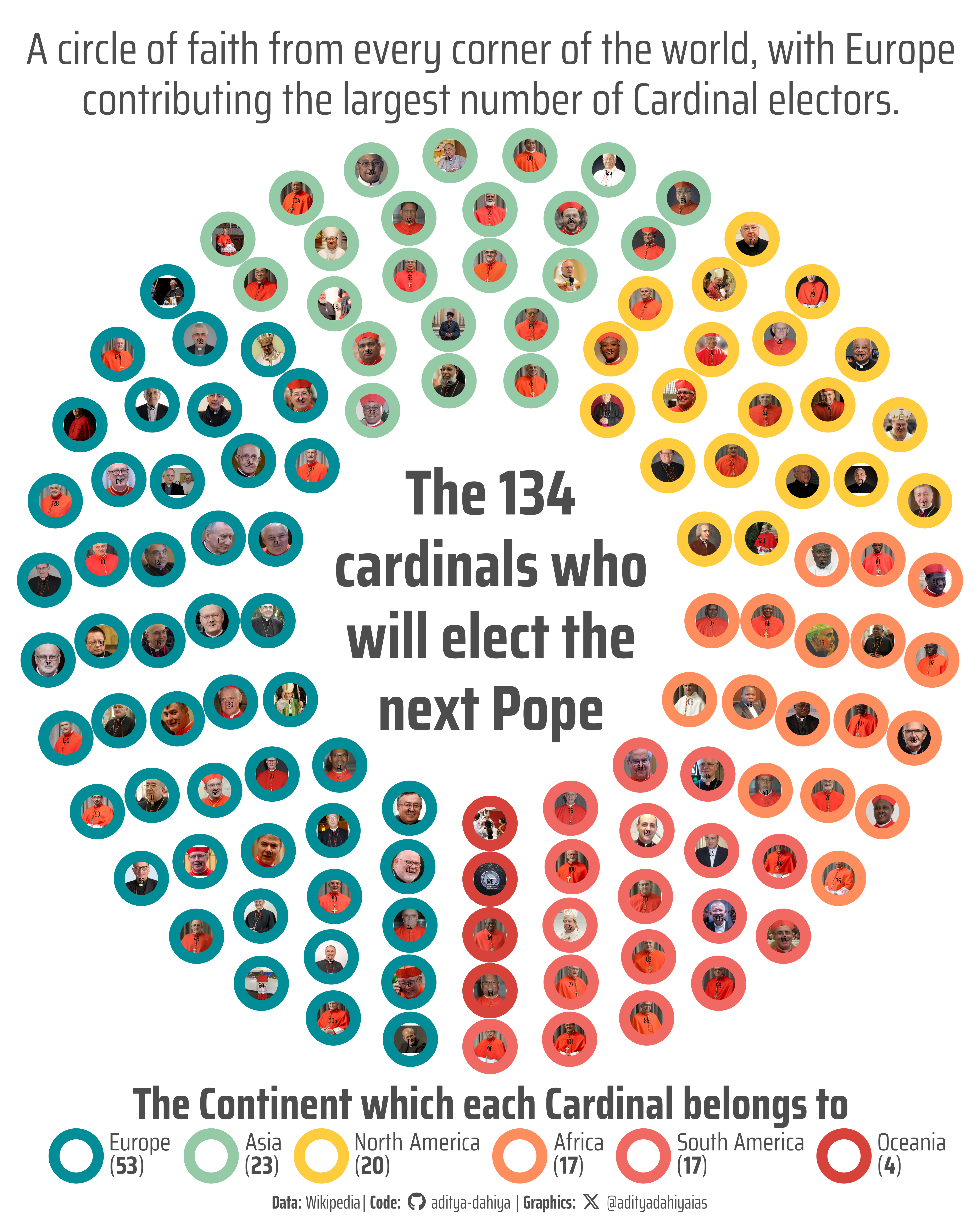
Who Will Choose the Next Pope?

Figure 1: This graphic shows the age distribution of the 134 cardinal electors for the 2025 papal conclave. Each dot represents a cardinal, placed according to their age. The colour of each dot indicates the cardinal’s continent — reflecting the dominance of Europe and the global nature of Roman Catholic Church. The visualization highlights the dynamics of geography which might come into play in the next Papal Conclave.

About the Data

The data for this visualization originates from the Wikipedia article Cardinal electors in the 2025 papal conclave, which provides a comprehensive and up-to-date list of the 135 cardinal electors eligible to participate in the upcoming conclave following the death of Pope Francis on April 21, 2025. This resource compiles information from official Vatican sources, including the Holy See Press Office and the Annuarium Statisticum Ecclesiae, and details each cardinal’s name, country, date of birth, ecclesiastical order (bishop, priest, or deacon), date of appointment (consistory), and the pope who appointed them. Notably, it also tracks changes in eligibility, such as Cardinal Antonio Cañizares Llovera’s decision not to attend due to health reasons, reducing the number of expected participants to 134. The dataset reflects the global composition of the College of Cardinals, with representation from 71 countries across six continents, and highlights that Pope Francis appointed 108 of the 135 electors, underscoring his significant influence on the Church’s future leadership. (Cardinal electors in the 2025 papal conclave)

How I made this graphic?

To create this visualization, I began by scraping data from Wikipedia using the {rvest} package’s read_html() and html_table() functions. After cleaning and wrangling the dataset with {tidyverse} tools like mutate() and {janitor}’s clean_names(), I calculated each cardinal’s age and organized them by continent. For the layout, I used the {ggparliament} package, especially its powerful parliament_data() function, to arrange the cardinals in a circular “parliament” style, grouped by continent and ordered by seniority. Portrait images of the cardinals were fetched using Google’s Custom Search API, processed with {magick} and {cropcircles} to create circular thumbnails. The final plot was crafted with {ggplot2}, where I used {ggimage}’s geom_image() to place each cardinal’s photo in the layout, enhanced the plot with customized fonts through {showtext}, markdown support via {ggtext}, and composed polished legends and captions. The colour palette was selected with {paletteer}. Careful attention was given to typography, accessibility, and design, resulting in a detailed and engaging visual story.

Loading required libraries

pacman::p_load(
  tidyverse,            # All things tidy
  
  scales,               # Nice Scales for ggplot2
  fontawesome,          # Icons display in ggplot2
  ggtext,               # Markdown text support for ggplot2
  showtext,             # Display fonts in ggplot2
  colorspace,           # Lighten and Darken colours
  
  magick,               # Download images and edit them
  ggimage,              # Display images in ggplot2
  patchwork,            # Composing Plots
  rvest,                # Web-Scraping
  ggbeeswarm,           # Beeswarm Plots
  ggparliament          # Parliament Layout computations
)


# URL of the Wikipedia page
# Read the HTML content of the page
page <- read_html("https://en.wikipedia.org/wiki/Cardinal_electors_in_the_2025_papal_conclave")

# Extract the first table (which contains the list of cardinals)
table_df <- page |> 
  html_table(fill = TRUE)
table_df <- table_df[[1]]

rm(page)

Visualization Parameters

# Font for titles
font_add_google("Saira",
  family = "title_font"
) 

# Font for the caption
font_add_google("Saira Extra Condensed",
  family = "caption_font"
) 

# Font for plot text
font_add_google("Saira Condensed",
  family = "body_font"
) 

showtext_auto()

# cols4all::c4a_gui()

mypal <- paletteer::paletteer_d("NineteenEightyR::sunset2")[c(5,3,1)]

# A base Colour
bg_col <- "white"
seecolor::print_color(bg_col)

# Colour for highlighted text
text_hil <- "grey30"
seecolor::print_color(text_hil)

# Colour for the text
text_col <- "grey30"
seecolor::print_color(text_col)

line_col <- "grey30"

# Define Base Text Size
bts <- 90

# Caption stuff for the plot
sysfonts::font_add(
  family = "Font Awesome 6 Brands",
  regular = here::here("docs", "Font Awesome 6 Brands-Regular-400.otf")
)
github <- "&#xf09b"
github_username <- "aditya-dahiya"
xtwitter <- "&#xe61b"
xtwitter_username <- "@adityadahiyaias"
social_caption_1 <- glue::glue("<span style='font-family:\"Font Awesome 6 Brands\";'>{github};</span> <span style='color: {text_hil}'>{github_username}  </span>")
social_caption_2 <- glue::glue("<span style='font-family:\"Font Awesome 6 Brands\";'>{xtwitter};</span> <span style='color: {text_hil}'>{xtwitter_username}</span>")
plot_caption <- paste0(
  "**Data:** Wikipedia", 
  " |  **Code:** ", 
  social_caption_1, 
  " |  **Graphics:** ", 
  social_caption_2
  )
rm(github, github_username, xtwitter, 
   xtwitter_username, social_caption_1, 
   social_caption_2)

# Add text to plot-------------------------------------------------
plot_title <- "The 134 cardinals who will elect the next Pope" |> str_wrap(15)
str_view(plot_title)

plot_subtitle <- "A circle of faith from every corner of the world, with Europe contributing the largest number of Cardinal electors." |> 
  str_wrap(65)
str_view(plot_subtitle)

Get temporary files on images of each Cardinal

# Get a custom google search engine and API key
# Tutorial: https://developers.google.com/custom-search/v1/overview
# Tutorial 2: https://programmablesearchengine.google.com/

# From:https://developers.google.com/custom-search/v1/overview
# google_api_key <- "LOAD YOUR GOOGLE API KEY HERE"

# From: https://programmablesearchengine.google.com/controlpanel/all
# my_cx <- "GET YOUR CUSTOM SEARCH ENGINE ID HERE"


# Improved function to download and save food images
download_cardinal_potrait <- function(i) {
  
  google_api_key <- google_api_key
  my_cx <- my_cx
  
  # Build the API request URL with additional filters
  url <- paste0(
    "https://www.googleapis.com/customsearch/v1?q=",
    URLencode(paste0("Cardinal ", cardinals$name[i], 
                     " photo")),
    "&cx=", my_cx,
    "&searchType=image",
    "&key=", google_api_key,
    # "&imgSize=large",       # Restrict to medium-sized images
    # "&imgType=photo",
    "&num=1"                 # Fetch only one result
  )
  
  # Make the request
  response <- httr::GET(url)
  # if (response$status_code != 200) {
  #   warning("Failed to fetch data for Cardinal: ", 
  #           cardinals$name[i])
  #   return(NULL)
  # }
  
  # Parse the response
  result <- httr::content(response, "parsed")
  
  # Extract the image URL
  image_url <- result$items[[1]]$link
  
  # Process the image
  magick::image_read(image_url) |> 
    image_resize("x300") |> 
    
    # Crop the image into a circle 
    # (Credits: https://github.com/doehm/cropcircles)
    cropcircles::circle_crop(
      border_colour = "black",
      border_size = 0
    ) |>
    
    image_read() |> 
    image_background(color = "transparent") |> 
    
    image_resize("x300") |> 
    
    # Save or display the result
    image_write(
      here::here(
        "data_vizs", 
        paste0("temp_cardinals_", i, ".png")
        )
    )
}

# Iterate and download images
for (i in 1:nrow(cardinals)) {
  download_cardinal_potrait(i)
}

problem_numbers <- c(5, 6,  7, 16, 32, 36, 73)

Exploratory Data Analysis and Wrangling

# Ensure the table is a tibble
cardinals <- as_tibble(table_df) |> 
  janitor::clean_names() |> 
  mutate(
    # Extract the date string from raw data
    born = str_extract(born, "^\\d{1,2} \\w+ \\d{4}"),
    # Convert to Date format
    born = dmy(born),  
    
    # Calculate age for each cardinal in years
    age = time_length(
      interval(
        start = born, 
        end = today()), 
        unit = "years") |> 
      floor()

  ) |> 
  mutate(
    date_consistory = str_extract(
      consistory, "^\\d{1,2} \\w+ \\d{4}"
      ) |>  dmy(),
    pope_consistory = str_remove(
      consistory, "^\\d{1,2} \\w+ \\d{4}"
      ) |>  str_trim(),
    pope_consistory = paste0("Pope ", pope_consistory),
    .keep = "unused"
  ) |> 
  select(-ref) |> 
  mutate(
    country = str_remove_all(country, "\\[.*?\\]"),
    order = fct(order, levels = c("CB", "CP", "CD"))
  )


plotdf2 <- cardinals |> 
  # Get ISO 3 code for countries, so that we can add continents
  mutate(
    country = if_else(country == "Jerusalem", "Israel", country),
    iso3c = countrycode::countrycode(
      country,
      origin = "country.name.en",
      destination = "iso3c"
    )
  ) |> 
  
  # Add continents based on countries
  left_join(
    rnaturalearth::ne_countries(returnclass = "sf") |> 
      sf::st_drop_geometry() |> 
      mutate(iso_a3 = if_else(name == "France", "FRA", iso_a3)) |> 
      select(iso_a3, continent) |> 
      rename(iso3c = iso_a3)
  ) |> 
  mutate(
    continent = case_when(
      iso3c == "CPV" ~ "Europe",
      iso3c == "MLT" ~ "Europe",
      iso3c == "SGP" ~ "Asia",
      iso3c == "HKG" ~ "Asia",
      iso3c == "TON" ~ "Oceania",
      .default = continent
    )
  ) |> 
  #select(rank, name, country, iso3c, continent, born, order, pope_consistory) |> 
  mutate(image_var = paste0("data_vizs/temp_cardinals_", rank, ".png"))

# plotdf2  |> 
#   count(continent, country)

# Continents Data
interact_legend <- plotdf3 |> 
  arrange(continent, country) |> 
  mutate(label1 = paste0(name, " (", country,")")) |> 
  group_by(continent) |> 
  mutate(label2 = row_number()) |> 
  summarise(
    label3 = paste0(label2, ". ", label1, collapse = "\n")
  )

get_legend_data <- function(x){
  interact_legend |> 
    filter(continent = x) |> 
    pull(label3)
}

Getting a parliament layout

# devtools::install_github("zmeers/ggparliament")
# pacman::p_load_gh("zmeers/ggparliament")

# The number of rows we want in the parliament layout
number_of_rows <- 5

# Continents count and their order
continent_counts_df <- plotdf2 |> 
  count(continent, sort = T) 
continent_df <- continent_counts_df |> 
  mutate(
    continent = fct(
      continent,
      levels = continent_counts_df$continent
    )
  )

# Improved plotdf2 for making cardinals in same orders: by continent and by rank
plotdf3 <- plotdf2 |> 
  mutate(
    continent = fct(
      continent,
      levels = continent_counts_df$continent
    )
  ) |> 
  arrange(continent, country, rank) |> 
  # An ID to link it up with ggpariament layout
  mutate(id = row_number()) |> 
  
  # Add the parliament layout data
  left_join(
    # Computate the parliament layout of Cardinals
    parliament_data(
      election_data = continent_df,
      # type = "semicircle",
      type = "circle",
      party_seats = continent_df$n,
      parl_rows = number_of_rows,
      plot_order = continent_df$continent
    ) |> 
      as_tibble() |> 
      
      # Now this gives layout where senior ranked Cardinals are away from the well.
      # I need to computate straight-line (Euclidean) distance from centre of circle 
      # (i.e. (0,0)) / semi-circle and get senior ranked caridnals near the well.
      mutate(
        depth = sqrt(x^2 + y^2),
        y_dist = y
      ) |> 
      arrange(continent, depth, y_dist) |> 
      mutate(
        id = row_number()
      )
  )

The Plot

g <- plotdf3 |> 
  ggplot(
    mapping = aes(
      x = x,
      y = y
    )
  ) +
  ggimage::geom_image(
    mapping = aes(image = image_var),
    size = 0.05
  ) +
  geom_point(
    mapping = aes(
      colour = continent
    ),
    size = 18,
    pch = 21,
    fill = NA,
    stroke = 9
  ) +
  geom_text(
    mapping = aes(
      label = rank
    ),
    colour = "black",
    family = "caption_font",
    hjust = 0.5,
    vjust = 1,
    lineheight = 0.25,
    size = bts / 10
  ) +
  annotate(
    geom = "text",
    label = plot_title,
    x = 0,
    y = 0,
    family = "body_font",
    size = bts * 0.9,
    hjust = 0.5,
    vjust = 0.5,
    lineheight = 0.3,
    colour = text_hil,
    fontface = "bold"
  ) +
  paletteer::scale_colour_paletteer_d(
    "MoMAColors::ustwo",
    direction = -1,
    labels = continent_df |> 
              mutate(label = paste0(continent, "<br>(**", n, "**)")) |> 
              pull(label)
    ) +
  coord_fixed(
    clip = "off"
  ) +
  guides(
    colour = guide_legend(
      nrow = 1
    )
  ) +
  labs(
    caption = plot_caption,
    colour = "The Continent which each Cardinal belongs to",
    y = NULL, x = NULL,
    subtitle = plot_subtitle
  ) +
  theme_void(
    base_family = "body_font",
    base_size = bts
  ) +
  theme(
    
    # Overall
    plot.margin = margin(5,0,2,0, "mm"),
    plot.title.position = "plot",
    
    text = element_text(
      colour = text_hil,
      lineheight = 0.3,
      hjust = 0.5
    ),
    
    # Labels and Strip Text
    plot.subtitle = element_text(
      colour = text_hil,
      margin = margin(5,0,-5,0, "mm"),
      size = bts * 1.8,
      lineheight = 0.3,
      hjust = 0.5
    ),
    plot.caption = element_textbox(
      margin = margin(3,0,0,0, "mm"),
      hjust = 0.5,
      colour = text_hil,
      size = 0.75 * bts,
      family = "caption_font"
    ),
    plot.caption.position = "plot",
    
    # Legend
    legend.position = "bottom",
    legend.margin = margin(1,1,1,1, "mm"),
    legend.box.margin = margin(0,0,0,0, "mm"),
    legend.title.position = "top",
    legend.title = element_text(
      margin = margin(-6,0,2,0, "mm"),
      hjust = 0.5,
      size = 1.8 * bts,
      face = "bold"
    ),
    legend.text = element_textbox(
      margin = margin(2,-9,2,5, "mm"),
      size = bts,
      hjust = 0.1
    ),
    legend.text.position = "right",
    legend.background = element_rect(
      fill = alpha(bg_col, 0.7),
      colour = NA
    )
  )

ggsave(
  filename = here::here(
    "data_vizs",
    "viz_papal_conclave_2025_parliament.png"
  ),
  plot = g,
  width = 400,
  height = 500,
  units = "mm",
  bg = bg_col
)

Savings the thumbnail for the webpage

# Saving a thumbnail

library(magick)

# Saving a thumbnail for the webpage
image_read(here::here("data_vizs", 
                      "viz_papal_conclave_2025_parliament.png")) |> 
  image_resize(geometry = "x400") |> 
  image_write(
    here::here(
      "data_vizs", 
      "thumbnails", 
      "viz_papal_conclave_2025_parliament.png"
    )
  )

Session Info

pacman::p_load(
  tidyverse,            # All things tidy
  
  scales,               # Nice Scales for ggplot2
  fontawesome,          # Icons display in ggplot2
  ggtext,               # Markdown text support for ggplot2
  showtext,             # Display fonts in ggplot2
  colorspace,           # Lighten and Darken colours
  
  magick,               # Download images and edit them
  ggimage,              # Display images in ggplot2
  patchwork,            # Composing Plots
  rvest,                # Web-Scraping
  ggbeeswarm,           # Beeswarm Plots
  ggparliament          # Parliament Layout computations
)

sessioninfo::session_info()$packages |> 
  as_tibble() |> 
  select(package, 
         version = loadedversion, 
         date, source) |> 
  arrange(package) |> 
  janitor::clean_names(
    case = "title"
  ) |> 
  gt::gt() |> 
  gt::opt_interactive(
    use_search = TRUE
  ) |> 
  gtExtras::gt_theme_espn()

Table 1: R Packages and their versions used in the creation of this page and graphics

Interactive Version

pacman::p_load(
  tidyverse,            # All things tidy
  
  scales,               # Nice Scales for ggplot2
  fontawesome,          # Icons display in ggplot2
  ggtext,               # Markdown text support for ggplot2
  showtext,             # Display fonts in ggplot2
  colorspace,           # Lighten and Darken colours
  
  magick,               # Download images and edit them
  ggimage,              # Display images in ggplot2
  patchwork,            # Composing Plots
  rvest,                # Web-Scraping
  ggbeeswarm,           # Beeswarm Plots
  ggparliament,         # Parliament Layout computations
  ggiraph               # Interactive Visualization
)

plot_title <- "The 134 cardinals who will elect the next Pope" |> str_wrap(15)

# A base Colour
bg_col <- "white"

# Colour for highlighted text
text_hil <- "grey30"

# Colour for the text
text_col <- "grey30"

line_col <- "grey30"


# Load Data --------------------------------------------------
# URL of the Wikipedia page
# Read the HTML content of the page
page <- read_html("https://en.wikipedia.org/wiki/Cardinal_electors_in_the_2025_papal_conclave")

# Extract the first table (which contains the list of cardinals)
table_df <- page |> 
  html_table(fill = TRUE)
table_df <- table_df[[1]]

rm(page)

# Data Wrangling --------------------------------------------

# Ensure the table is a tibble
cardinals <- as_tibble(table_df) |> 
  janitor::clean_names() |> 
  mutate(
    # Extract the date string from raw data
    born = str_extract(born, "^\\d{1,2} \\w+ \\d{4}"),
    # Convert to Date format
    born = dmy(born),  
    
    # Calculate age for each cardinal in years
    age = time_length(
      interval(
        start = born, 
        end = today()), 
        unit = "years") |> 
      floor()

  ) |> 
  mutate(
    date_consistory = str_extract(
      consistory, "^\\d{1,2} \\w+ \\d{4}"
      ) |>  dmy(),
    pope_consistory = str_remove(
      consistory, "^\\d{1,2} \\w+ \\d{4}"
      ) |>  str_trim(),
    pope_consistory = paste0("Pope ", pope_consistory),
    .keep = "unused"
  ) |> 
  select(-ref) |> 
  mutate(
    country = str_remove_all(country, "\\[.*?\\]"),
    order = fct(order, levels = c("CB", "CP", "CD"))
  )


plotdf2 <- cardinals |> 
  # Get ISO 3 code for countries, so that we can add continents
  mutate(
    country = if_else(country == "Jerusalem", "Israel", country),
    iso3c = countrycode::countrycode(
      country,
      origin = "country.name.en",
      destination = "iso3c"
    )
  ) |> 
  
  # Add continents based on countries
  left_join(
    rnaturalearth::ne_countries(returnclass = "sf") |> 
      sf::st_drop_geometry() |> 
      mutate(iso_a3 = if_else(name == "France", "FRA", iso_a3)) |> 
      select(iso_a3, continent) |> 
      rename(iso3c = iso_a3)
  ) |> 
  mutate(
    continent = case_when(
      iso3c == "CPV" ~ "Europe",
      iso3c == "MLT" ~ "Europe",
      iso3c == "SGP" ~ "Asia",
      iso3c == "HKG" ~ "Asia",
      iso3c == "TON" ~ "Oceania",
      .default = continent
    )
  ) |> 
  #select(rank, name, country, iso3c, continent, born, order, pope_consistory) |> 
  mutate(image_var = paste0("data_vizs/temp_cardinals_", rank, ".png"))

# plotdf2  |> 
#   count(continent, country)

# Parliament Layout -----------------------------------------------

# The number of rows we want in the parliament layout
number_of_rows <- 5

# Continents count and their order
continent_counts_df <- plotdf2 |> 
  count(continent, sort = T) 
continent_df <- continent_counts_df |> 
  mutate(
    continent = fct(
      continent,
      levels = continent_counts_df$continent
    )
  )

# Improved plotdf2 for making cardinals in same orders: by continent and by rank
plotdf3 <- plotdf2 |> 
  mutate(
    continent = fct(
      continent,
      levels = continent_counts_df$continent
    )
  ) |> 
  arrange(continent, country, rank) |> 
  # An ID to link it up with ggpariament layout
  mutate(id = row_number()) |> 
  
  # Add the parliament layout data
  left_join(
    # Computate the parliament layout of Cardinals
    parliament_data(
      election_data = continent_df,
      # type = "semicircle",
      type = "circle",
      party_seats = continent_df$n,
      parl_rows = number_of_rows,
      plot_order = continent_df$continent
    ) |> 
      as_tibble() |> 
      
      # Now this gives layout where senior ranked Cardinals are away from the well.
      # I need to computate straight-line (Euclidean) distance from centre of circle 
      # (i.e. (0,0)) / semi-circle and get senior ranked caridnals near the well.
      mutate(
        depth = sqrt(x^2 + y^2),
        y_dist = y
      ) |> 
      arrange(continent, depth, y_dist) |> 
      mutate(
        id = row_number()
      )
  )

# Data for interactive Legend -------------------------------------

# Continents Data
interact_legend <- plotdf3 |> 
  arrange(continent, country) |> 
  mutate(label1 = paste0(name, " (", country,")")) |> 
  group_by(continent) |> 
  mutate(label2 = row_number()) |> 
  summarise(
    label3 = paste0(label2, ". ", label1, collapse = "\n")
  )

get_legend_data <- function(x){
  interact_legend |> 
    filter(continent == x) |> 
    pull(label3)
}

# VISUALIZATION ---------------------------------------------------

bts = 24
mypal <- paletteer::paletteer_d(
  "MoMAColors::ustwo", 
  direction = -1
  ) |> 
  as.character()
names(mypal) <- continent_df |> pull(continent)

g <- plotdf3 |> 
  ggplot(
    mapping = aes(
      x = x,
      y = y,
      data_id = id
    )
  ) +
  geom_point_interactive(
    mapping = aes(
      colour = continent,
      tooltip = paste0(
        "Name: ", name, "\n",
        "Office: ", office, "\n",
        "Country: ", country, "\n",
        "Continent: ", continent, "\n",
        "Age: ", age, " years\n",
        "Rank / Seniority: ", rank 
      )
    ),
    size = 22,
    pch = 20
  ) +
  annotate(
    geom = "text",
    label = plot_title,
    x = 0,
    y = 0,
    # family = "body_font",
    size = bts * 0.5,
    hjust = 0.5,
    vjust = 0.5,
    lineheight = 0.9,
    colour = text_hil,
    fontface = "bold"
  ) +
  scale_colour_manual_interactive(
    values = mypal,
    labels = continent_df |> 
              mutate(label = paste0(
                continent, "<br>(**", n, "**)")) |> 
              pull(label),
    data_id = function(x) x,
    tooltip = get_legend_data
    ) +
  coord_fixed(
    clip = "off"
  ) +
  labs(
    caption = "Data:Wikipedia   |    Code & Graphics: X @adityadahiyaias",
    colour = "The Continent which each Cardinal belongs to",
    y = NULL, x = NULL
  ) +
  theme_void(
    base_size = bts
  ) +
  theme(
    
    # Overall
    plot.margin = margin(5,0,2,0, "mm"),
    plot.title.position = "plot",
    
    text = element_text(
      colour = text_hil,
      hjust = 0.5
    ),
    
    # Labels and Strip Text
    plot.caption = element_textbox(
      hjust = 0.5,
      colour = text_hil,
      size = 0.6 * bts,
      margin = margin(3,0,1,0, "lines")
    ),
    plot.caption.position = "plot",
    
    # Legend
    legend.position = "bottom",
    legend.title.position = "top",
    legend.title = element_text(
      hjust = 0.5,
      face = "bold"
    ),
    legend.text = element_textbox(
      hjust = 0.1
    ),
    legend.text.position = "right"
  )

tooltip_css <- "background-color:white;color:black"

# INTERACTIVITY ----------------------------------------------------

girafe(
  ggobj = g,
  options = list(
    opts_tooltip(
      css = tooltip_css, 
      opacity = 0.9
      ),
    opts_sizing(width = .7),
    opts_hover_inv(css = "opacity:0.25;"),
    opts_hover(css = "fill:white;stroke:black;"),
    opts_zoom(max = 5)
  )
)

An interactive visualization on Cardinal Electors for the Papal Conclave 2025: A circle of faith from every corner of the world, with Europe contributing the largest number.