Global Mapping: UTM Zones Explained

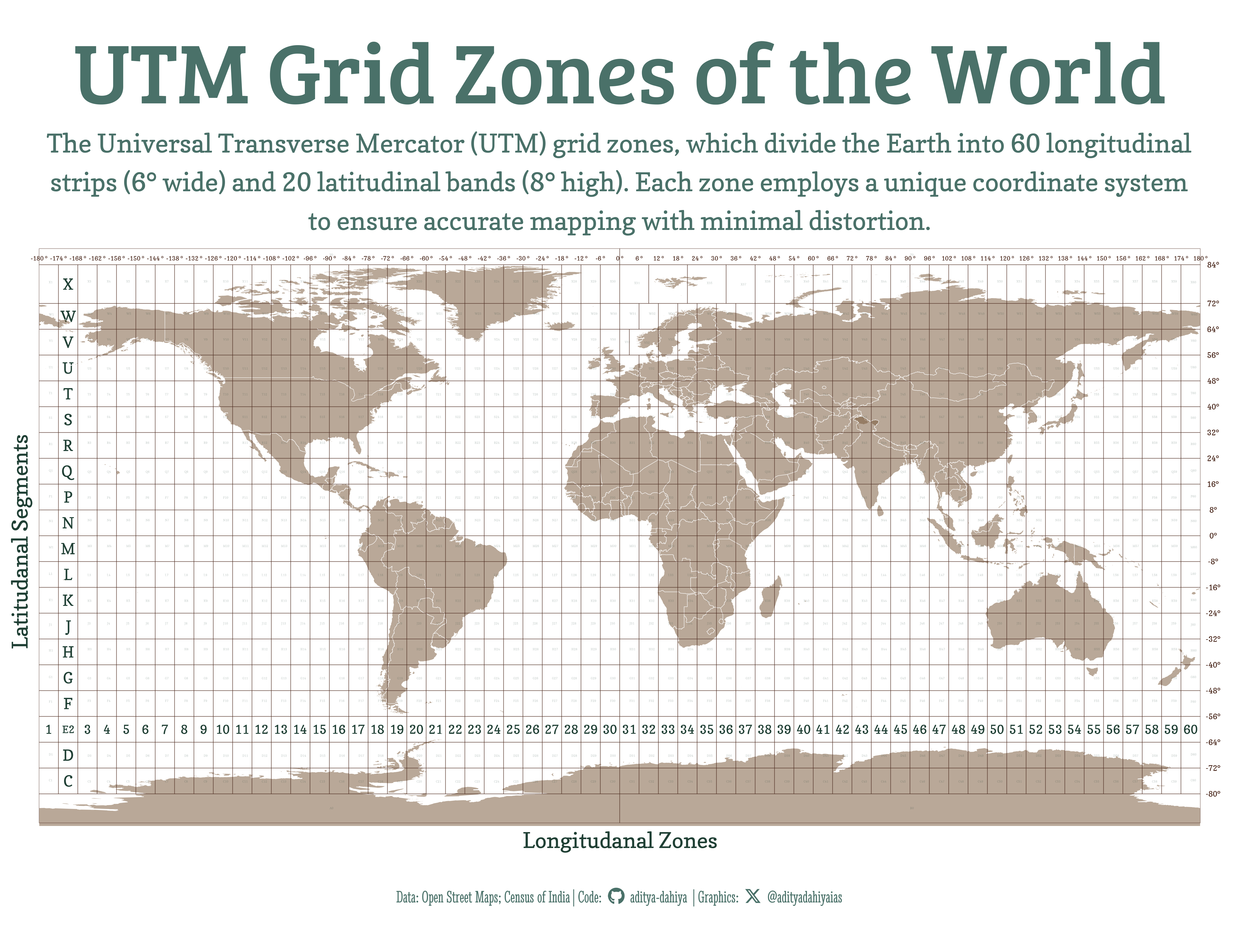
A global visualization of UTM zones, showcasing latitudinal bands labeled from C to X and longitudinal strips numbered 1 to 60, forming a precise grid for geospatial reference.

Figure 1: A global visualization of UTM zones, showcasing latitudinal bands labeled from C to X and longitudinal strips numbered 1 to 60, forming a precise grid for geospatial reference.

How I made this graphic?

Loading required libraries, data import & creating custom functions.

# Data Wrangling & Plotting Tools
library(tidyverse)            # All things tidy
library(sf)                   # Simple Features in R

# Plot touch-up tools
library(scales)               # Nice Scales for ggplot2
library(fontawesome)          # Icons display in ggplot2
library(ggtext)               # Markdown text support for ggplot2
library(showtext)             # Display fonts in ggplot2
library(colorspace)           # Lighten and Darken colours
library(patchwork)            # Compiling Plots

Visualization Parameters

# Font for titles
font_add_google("Bree Serif",
  family = "title_font"
) 

# Font for the caption
font_add_google("Stint Ultra Condensed",
  family = "caption_font"
) 

# Font for plot text
font_add_google("Copse",
  family = "body_font"
) 

showtext_auto()

mypal <- paletteer::paletteer_d("lisa::C_M_Coolidge")

# A base Colour
bg_col <- "white"
seecolor::print_color(bg_col)

land_col <- mypal[4]
seecolor::print_color(land_col)

# Colour for highlighted text - 1
text_hil1 <- mypal[2]
seecolor::print_color(text_hil1)

# Colour for the text - 1
text_col1 <- mypal[1]
seecolor::print_color(text_col1)


# Colour for highlighted text - 2
text_hil2 <- mypal[4]
seecolor::print_color(text_hil2)

# Colour for the text - 2
text_col2 <- mypal[5]
seecolor::print_color(text_col2)

# Define Base Text Size
bts <- 80 

# Caption stuff for the plot
sysfonts::font_add(
  family = "Font Awesome 6 Brands",
  regular = here::here("docs", "Font Awesome 6 Brands-Regular-400.otf")
)
github <- "&#xf09b"
github_username <- "aditya-dahiya"
xtwitter <- "&#xe61b"
xtwitter_username <- "@adityadahiyaias"
social_caption_1 <- glue::glue("<span style='font-family:\"Font Awesome 6 Brands\";'>{github};</span> <span style='color: {text_hil1}'>{github_username}  </span>")
social_caption_2 <- glue::glue("<span style='font-family:\"Font Awesome 6 Brands\";'>{xtwitter};</span> <span style='color: {text_hil1}'>{xtwitter_username}</span>")
plot_caption <- paste0(
  "**Data:** Open Street Maps; Census of India", 
  " |  **Code:** ", 
  social_caption_1, 
  " |  **Graphics:** ", 
  social_caption_2
  )
rm(github, github_username, xtwitter, 
   xtwitter_username, social_caption_1, 
   social_caption_2)

# Add text to plot-------------------------------------------------
plot_title <- "UTM Grid Zones of the World"

plot_subtitle <- "The Universal Transverse Mercator (UTM) grid zones, which divide the Earth into 60 longitudinal strips (6° wide) and 20 latitudinal bands (8° high). Each zone employs a unique coordinate system to ensure accurate mapping with minimal distortion."

Create data for the UTM Zones

india_map <- read_sf(
  here::here("data", "india_map", "India_Country_Boundary.shp")
) |> 
  st_simplify(dTolerance = 2000)

world_map <- rnaturalearth::ne_countries(
  scale = "large",
  returnclass = "sf"
) |> 
  select(name, geometry)

object.size(world_map) |> 
  print(units = "Mb")

# Create a tibble for the UTM Zone breaks
# First, the longitude breaks -------------------------------------------------
utm_long_breaks <- tibble(
  Longitude_Start = seq(-180, 174, by = 6),
  Longitude_End = seq(-174, 180, by = 6),
  Zone_Number = seq(1, 60)
) |> 
  janitor::clean_names() |>
  mutate(
    mid_point_long = (longitude_start + longitude_end)/2
  )

vlines <- tibble(
  vline_values = unique(
  c(utm_long_breaks$longitude_end, 
    utm_long_breaks$longitude_start)
  ) |> 
  sort()
)


# Then, the latitude breaks ---------------------------------------------------
utm_lat_breaks <- tibble(
  Latitude_Start = c(seq(-80, 72, by = 8)),
  Latitude_End = c(seq(-72, 72, by = 8), 84),
  Zone_Letter = LETTERS[!(LETTERS %in% c("A", "B", "I", "O", "Y", "Z"))]
) |> 
  janitor::clean_names() |>
  mutate(
    mid_point_lat = (latitude_start + latitude_end)/2
  )

hlines <- tibble(
  hline_values = unique(
  c(utm_lat_breaks$latitude_end, 
    utm_lat_breaks$latitude_start)
  ) |> 
  sort()
)

# Using the power of tidyr::crossing() to generate all zone names
zone_names <- crossing(
  utm_lat_breaks |> 
    select(zone_letter, mid_point_lat) |> 
    rename(lat_zone  = zone_letter, lat = mid_point_lat),

  utm_long_breaks |> 
    select(zone_number, mid_point_long) |> 
    rename(long_zone = zone_number, long = mid_point_long)
)

The Base Plot - an inaccurate approximation of the Zone Lines

g <- ggplot() +
  
  # Longitudes: Lines, Zone Labels and Longitude values ------------------------
  geom_segment(
    data = vlines,
    mapping = aes(
      x = vline_values,
      xend = vline_values,
      y = -96,
      yend = 86
    ),
    linewidth = 0.2,
    linetype = 1,
    colour = text_hil2,
    alpha = 0.3
  ) +

  # Longitude: Zone Labels
  geom_text(
    data = utm_long_breaks,
    mapping = aes(
      label = zone_number,
      y = -94,
      x = mid_point_long
    ),
    family = "body_font",
    size = bts / 5,
    colour = text_col1,
    fontface = "bold"
  ) +
  
  # Longitude: The actual values of longitude
  geom_text(
    data = vlines,
    mapping = aes(
      label = paste(vline_values, "°"),
      x = vline_values,
      y = 90
    ),
    family = "body_font",
    size = bts / 10,
    colour = text_col2
  ) +
  
  # Latitudes: Lines, Zone Labels, and Latitude Values -------------------------
  # Latitude: Zone Labels
  geom_text(
    data = utm_lat_breaks,
    mapping = aes(
      label = zone_letter,
      x = -184,
      y = mid_point_lat
    ),
    family = "body_font",
    size = bts / 4,
    colour = text_col1,
    fontface = "bold"
  ) +
  
  # Latitude Lines
  geom_segment(
    data = hlines,
    mapping = aes(
      y = hline_values, yend = hline_values,
      x = -184, xend = 182
    ),
    linewidth = 0.2,
    linetype = 1,
    colour = text_hil2,
    alpha = 0.3
  ) + 
  
  # Latitude actual values to display
  geom_text(
    data = hlines,
    mapping = aes(
      label = paste0(hline_values, "°"),
      y = hline_values,
      x = 186
    ),
    family = "body_font",
    size = bts / 8,
    colour = text_col2
  ) +
  
  # The World Map
  geom_sf(
    data = world_map |> filter(name != "India"),
    alpha = 0.5,
    colour = "white",
    fill = alpha(land_col, 0.4)
  ) +
  geom_sf(
    data = india_map,
    alpha = 0.5,
    colour = "white",
    fill = alpha(land_col, 0.4)
  ) +
  
  # Displaying zone names
  geom_text(
    data = zone_names,
    mapping = aes(
      label = paste0(lat_zone, long_zone),
      x = long, y = lat
    ),
    size = bts / 20,
    colour = alpha(text_hil2, 0.4),
    family = "body_font",
    hjust = 0,
    vjust = 0,
    nudge_x = -2.4,
    nudge_y = -3.4
  ) +
  
  # Coordinates
  coord_sf(
    expand = FALSE,
    clip = "off"
  ) +
  
  # Labels and Themes
  labs(
    x = "Longitudanal Zones",
    y = "Latitudanal Segments",
    title = plot_title,
    subtitle = str_wrap(plot_subtitle, 100),
    caption = plot_caption
  ) +
  ggthemes::theme_map(
    base_family = "body_font",
    base_size = bts
  ) +
  theme(
    
    # Full plot features
    plot.margin = margin(15,5,15,5, "mm"),
    panel.grid = element_blank(),
    axis.text = element_blank(),
    axis.ticks = element_blank(),
    axis.ticks.length = unit(0, "mm"),
    axis.title = element_text(
      family = "body_font",
      margin = margin(0,0,0,0, "mm"),
      colour = text_col1
    ),
    plot.title.position = "plot",
    text = element_text(
      colour = text_col2
    ),
    
    # Labels and titles
    plot.title = element_text(
      hjust = 0.5,
      size = 4 * bts,
      family = "title_font",
      lineheight = 0.3,
      margin = margin(0,0,5,0, "mm"),
      colour = text_hil1
    ),
    plot.subtitle = element_text(
      hjust = 0.5,
      size = 1.2 * bts,
      family = "body_font",
      lineheight = 0.4,
      margin = margin(0,0,10,0, "mm"),
      colour = text_hil1
    ),
    plot.caption = element_textbox(
      hjust = 0.5,
      family = "caption_font",
      lineheight = 0.3,
      margin = margin(15,0,0,0, "mm"),
      size = 0.8 * bts,
      colour = text_hil1
    )
  )

ggsave(
  filename = here::here(
    "data_vizs",
    "viz_utm_zones.png"
  ),
  plot = g,
  width = 500,
  height = 400,
  units = "mm",
  bg = bg_col
)

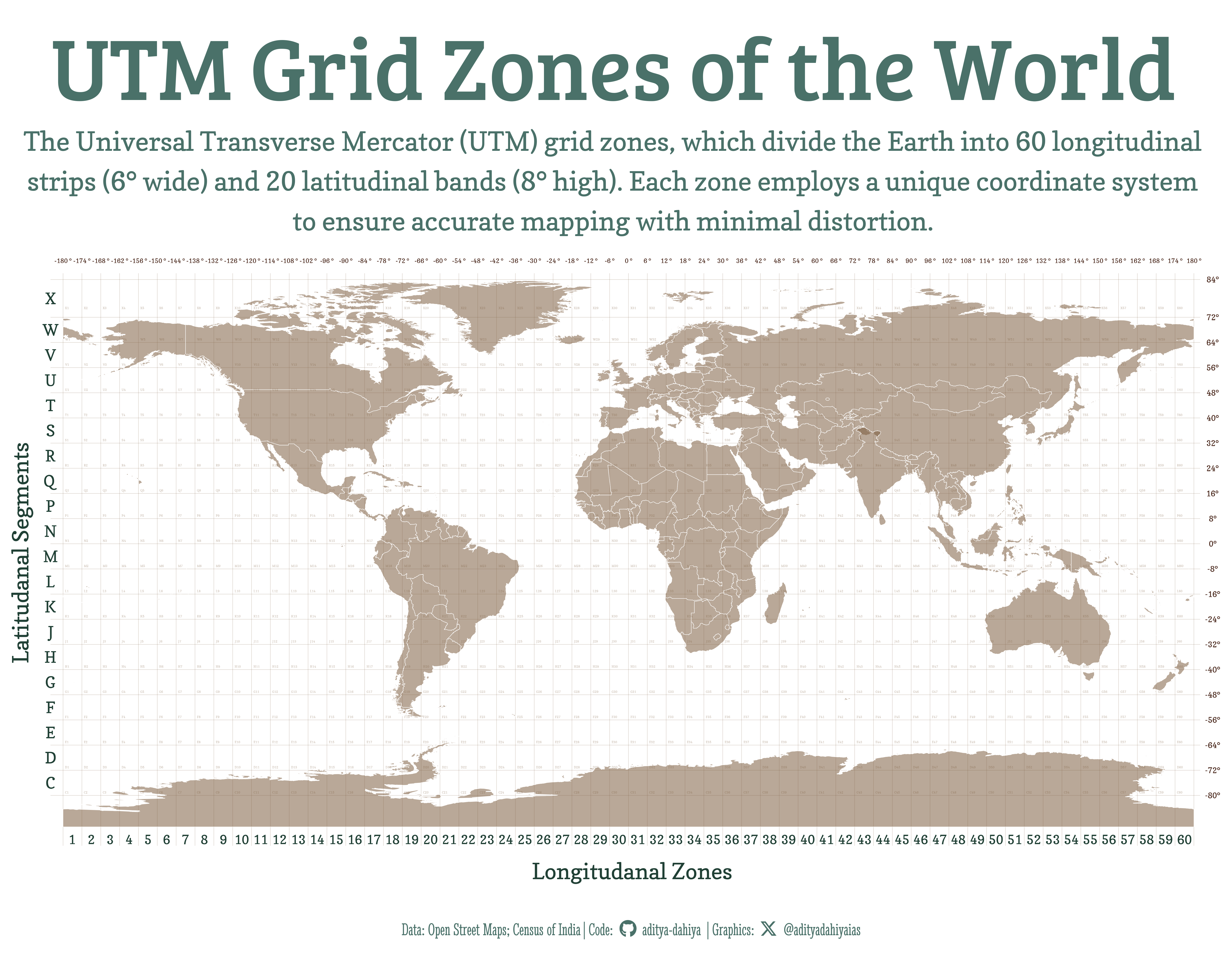
A global visualization of UTM zones, showcasing latitudinal bands labeled from C to X and longitudinal strips numbered 1 to 60, forming a precise grid for geospatial reference.

Another more accurate attempt: the Final Visualization

utm_zones <- read_sf(
  here::here(
    "data",
    "world_utm_grid_arcgis.gpkg"
  )
) |> 
  janitor::clean_names()


g <- ggplot() +
  
  # Longitude: Zone Labels
  geom_text(
    data = utm_long_breaks |> filter(zone_number != 2),
    mapping = aes(
      label = zone_number,
      y = -60,
      x = mid_point_long
    ),
    family = "body_font",
    size = bts / 5,
    colour = text_col1,
    fontface = "bold",
    vjust = 0.5, hjust = 0.5
  ) +
  
  # Longitude: Degree Values
  geom_text(
    data = vlines,
    mapping = aes(
      label = paste(vline_values, "°"),
      x = vline_values,
      y = 86
    ),
    family = "body_font",
    size = bts / 10,
    colour = text_col2
  ) +
  
  # Latitude: Zone Labels
  geom_text(
    data = utm_lat_breaks |> filter(zone_letter != "E"),
    mapping = aes(
      label = zone_letter,
      x = -171,
      y = mid_point_lat
    ),
    family = "body_font",
    size = bts / 4,
    colour = text_col1,
    fontface = "bold",
    hjust = 0.5, vjust = 0.5
  ) +
  
  # Add a custom label for E2
  geom_text(
    data = tibble(zone_letter = "E2"),
    mapping = aes(
      label = zone_letter,
      x = -171,
      y = -60
    ),
    family = "body_font",
    size = bts / 6,
    colour = text_col1,
    fontface = "bold",
    hjust = 0.5, vjust = 0.5
  ) +
  
  # Latitude: Degree Values
  geom_text(
    data = hlines,
    mapping = aes(
      label = paste0(hline_values, "°"),
      y = hline_values,
      x = 184
    ),
    family = "body_font",
    size = bts / 8,
    colour = text_col2
  ) +
  
  # The World Map
  geom_sf(
    data = world_map |> filter(name != "India"),
    alpha = 0.5,
    colour = "white",
    fill = alpha(land_col, 0.4)
  ) +
  
  geom_sf(
    data = india_map,
    alpha = 0.5,
    colour = "white",
    fill = alpha(land_col, 0.4)
  ) +
  
  # Displaying UTM Zones and their names
  geom_sf(
    data = utm_zones,
    linewidth = 0.3,
    colour = alpha(text_col2, 0.5),
    fill = NA
  ) +
  geom_sf_text(
    data = utm_zones |> filter(zone != 2) |> filter(row != "E"),
    mapping = aes(
      label = paste0(row, zone)
    ),
    family = "body_font",
    colour = alpha(text_col1, 0.25),
    hjust = 0,
    vjust = 0,
    fontface = "bold"
  ) +
  
  
  # Coordinates
  coord_sf(
    expand = FALSE,
    clip = "off",
    xlim = c(-188, 188),
    ylim = c(-86, 82),
    default_crs = "EPSG:4326"
  ) +
  
  # Labels and Themes
  labs(
    x = "Longitudanal Zones",
    y = "Latitudanal Segments",
    title = plot_title,
    subtitle = str_wrap(plot_subtitle, 100),
    caption = plot_caption
  ) +
  ggthemes::theme_map(
    base_family = "body_font",
    base_size = bts
  ) +
  theme(
    
    # Full plot features
    plot.margin = margin(15,5,15,5, "mm"),
    panel.grid = element_blank(),
    axis.text = element_blank(),
    axis.ticks = element_blank(),
    axis.ticks.length = unit(0, "mm"),
    axis.title.x = element_text(
      family = "body_font",
      margin = margin(8,0,0,0, "mm"),
      colour = text_col1
    ),
    axis.title.y = element_text(
      family = "body_font",
      margin = margin(0,-8,0,0, "mm"),
      colour = text_col1
    ),
    plot.title.position = "plot",
    text = element_text(
      colour = text_col2
    ),
    
    # Labels and titles
    plot.title = element_text(
      hjust = 0.5,
      size = 4 * bts,
      family = "title_font",
      lineheight = 0.3,
      margin = margin(0,0,5,0, "mm"),
      colour = text_hil1
    ),
    plot.subtitle = element_text(
      hjust = 0.5,
      size = 1.2 * bts,
      family = "body_font",
      lineheight = 0.4,
      margin = margin(0,0,15,0, "mm"),
      colour = text_hil1
    ),
    plot.caption = element_textbox(
      hjust = 0.5,
      family = "caption_font",
      lineheight = 0.3,
      margin = margin(15,0,0,0, "mm"),
      size = 0.8 * bts,
      colour = text_hil1
    )
  )

ggsave(
  filename = here::here(
    "data_vizs",
    "viz_utm_zones_2.png"
  ),
  plot = g,
  width = 520,
  height = 400,
  units = "mm",
  bg = bg_col
)

Savings the thumbnail for the webpage

# Saving a thumbnail

library(magick)
# Saving a thumbnail for the webpage
image_read(here::here("data_vizs", 
                      "viz_utm_zones.png")) |> 
  image_resize(geometry = "x400") |> 
  image_write(
    here::here(
      "data_vizs", 
      "thumbnails", 
      "viz_utm_zones.png"
    )
  )

Session Info

# Data Wrangling & Plotting Tools
library(tidyverse)            # All things tidy
library(sf)                   # Simple Features in R

# Plot touch-up tools
library(scales)               # Nice Scales for ggplot2
library(fontawesome)          # Icons display in ggplot2
library(ggtext)               # Markdown text support for ggplot2
library(showtext)             # Display fonts in ggplot2
library(colorspace)           # Lighten and Darken colours
library(patchwork)            # Compiling Plots

sessioninfo::session_info()$packages |> 
  as_tibble() |> 
  select(package, 
         version = loadedversion, 
         date, source) |> 
  arrange(package) |> 
  janitor::clean_names(
    case = "title"
  ) |> 
  gt::gt() |> 
  gt::opt_interactive(
    use_search = TRUE
  ) |> 
  gtExtras::gt_theme_espn()

Table 1: R Packages and their versions used in the creation of this page and graphics

An attempt at an Interactive Version

# A map with utm zones and countries falling in it
world_map <- rnaturalearth::ne_countries(
  scale = "small",
  returnclass = "sf"
) |> 
  select(name, geometry) |> 
  st_transform("EPSG:4326")


utm_zones <- read_sf(
  here::here(
    "data",
    "world_utm_grid_arcgis.gpkg"
  )
) |> 
  janitor::clean_names() |> 
  mutate(id = row_number()) |> 
  st_transform("EPSG:4326")


utm_zones |> 
  slice_head(n = 5)

# Data Wrangling & Plotting Tools
library(tidyverse)            # All things tidy
library(sf)                   # Simple Features in R
library(ggiraph)              # Interactive Plots

world_map <- rnaturalearth::ne_countries(
  scale = "large",
  returnclass = "sf"
) |> 
  select(name, geometry)


utm_zones <- read_sf(
  here::here(
    "data",
    "world_utm_grid_arcgis.gpkg"
  )
) |> 
  janitor::clean_names() |> 
  mutate(id = row_number())


g <- ggplot() +
  
  # Displaying UTM Zones
  geom_sf_interactive(
    data = utm_zones,
    mapping = aes(
      tooltip = paste0(row, zone),
      data_id = id
    ),
    linewidth = 0.15,
    colour = alpha(text_hil2, 0.5),
    fill = NA
  ) +
  
  # The World Map
  geom_sf(
    data = world_map,
    alpha = 0.5,
    colour = alpha(land_col, 0.4),
    fill = alpha(land_col, 0.4),
    linewidth = 0.2
  ) +
  
  # Coordinates
  coord_sf(
    crs = "EPSG:4326",
    expand = FALSE,
    clip = "off",
    xlim = c(-188, 188),
    ylim = c(-86, 86),
    default_crs = "EPSG:4326"
  ) +
  
  # Labels and Themes
  labs(
    x = "Longitudanal Zones",
    y = "Latitudanal Segments",
    title = plot_title,
    subtitle = str_wrap(plot_subtitle, 150)
  ) +
  ggthemes::theme_map() +
  theme(
    text = element_text(
      colour = text_hil2
    )
  )

girafe(
  ggobj = g
)