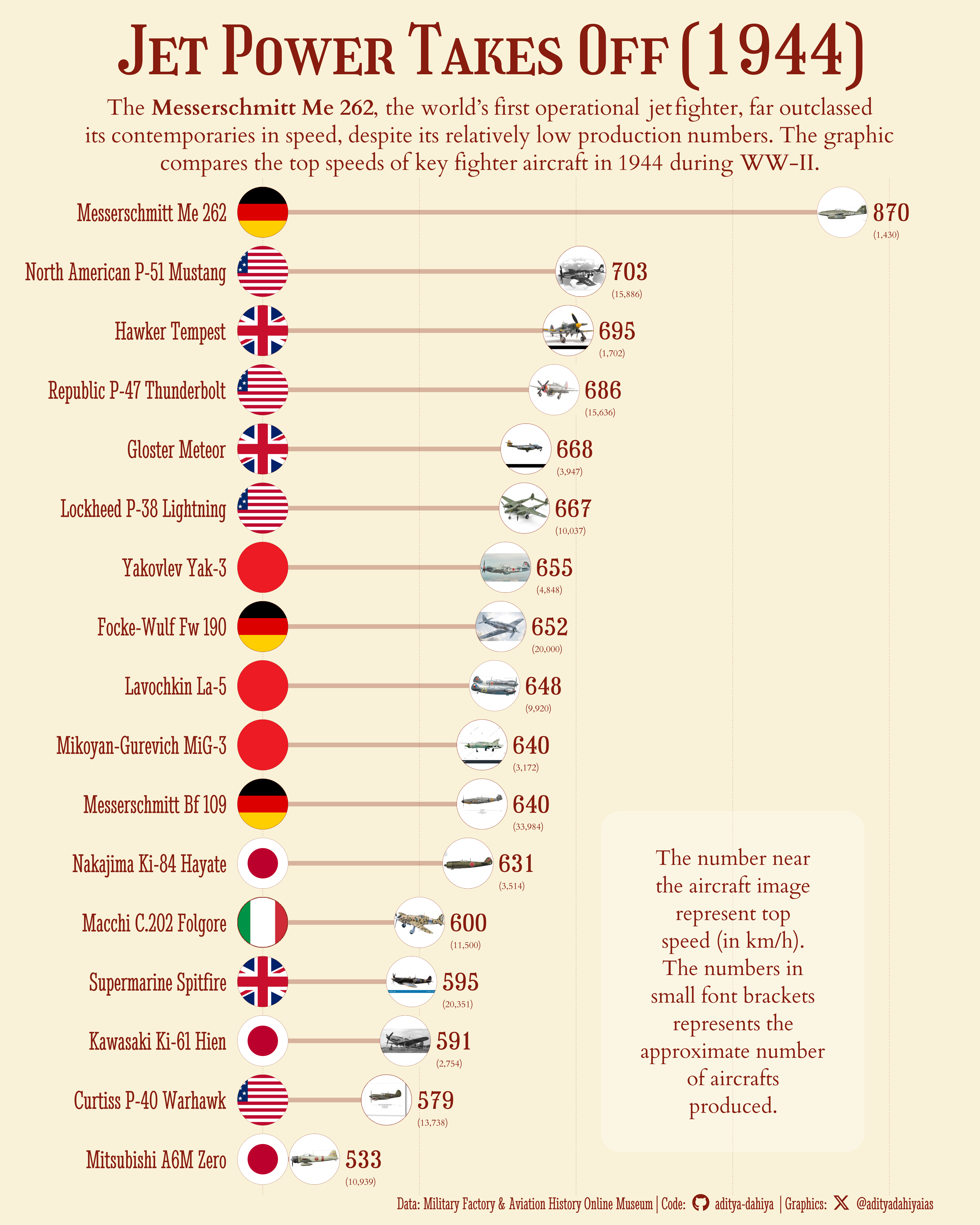
A visual comparison of top speeds and production numbers of World War II fighter aircraft reveals the Messerschmitt Me 262’s unmatched dominance in speed, marking a revolutionary leap in aviation technology during its era.
{magick}
Images
Geopolitics
Author
Aditya Dahiya
Published
January 28, 2025
Figure 1: This graphic visualizes the top speeds of WWII fighter aircraft at the time of the Messerschmitt Me 262’s introduction, with aircraft names listed on the y-axis in descending order of speed. The x-axis represents top speed (in km/h), and each bar includes the approximate production numbers in parentheses. Country flags are placed near the y-axis for easy identification, and accompanying aircraft images provide a visual connection to these iconic machines.
Source of Data
The information provided is compiled using ChatGPT from the following sources:
“The Complete Book of Fighters” by William Green and Gordon Swanborough
“Jane’s Fighting Aircraft of World War II” by Leonard Bridgman.
# Font for titlesfont_add_google("Girassol",family ="title_font") # Font for the captionfont_add_google("Stint Ultra Condensed",family ="caption_font") # Font for plot textfont_add_google("Cardo",family ="body_font") showtext_auto()mypal <- paletteer::paletteer_d("MexBrewer::Revolucion")# A base Colourbg_col <- mypal[5]seecolor::print_color(bg_col)# Colour for highlighted text - 1text_hil <- mypal[1]seecolor::print_color(text_hil)# Colour for the text - 1text_col <- mypal[1]seecolor::print_color(text_col)# Define Base Text Sizebts <-80# Caption stuff for the plotsysfonts::font_add(family ="Font Awesome 6 Brands",regular = here::here("docs", "Font Awesome 6 Brands-Regular-400.otf"))github <-""github_username <-"aditya-dahiya"xtwitter <-""xtwitter_username <-"@adityadahiyaias"social_caption_1 <- glue::glue("<span style='font-family:\"Font Awesome 6 Brands\";'>{github};</span> <span style='color: {text_hil}'>{github_username} </span>")social_caption_2 <- glue::glue("<span style='font-family:\"Font Awesome 6 Brands\";'>{xtwitter};</span> <span style='color: {text_hil}'>{xtwitter_username}</span>")plot_caption <-paste0("**Data:** Military Factory & Aviation History Online Museum", " | **Code:** ", social_caption_1, " | **Graphics:** ", social_caption_2 )rm(github, github_username, xtwitter, xtwitter_username, social_caption_1, social_caption_2)# Add text to plot-------------------------------------------------plot_title <-"Jet Power Takes Off (1944)"plot_subtitle <-str_wrap("The **Messerschmitt Me 262**, the world’s first operational jet fighter, far outclassed its contemporaries in speed, despite its relatively low production numbers. The graphic compares the top speeds of key fighter aircraft in 1944 during WW-II.", 90) |>str_replace_all("\\\n", "<br>")
Download images of the fighter aircraft
Code
# Get a custom google search engine and API key# Tutorial: https://developers.google.com/custom-search/v1/overview# Tutorial 2: https://programmablesearchengine.google.com/# From:https://developers.google.com/custom-search/v1/overview# google_api_key <- "LOAD YOUR GOOGLE API KEY HERE"# From: https://programmablesearchengine.google.com/controlpanel/all# my_cx <- "GET YOUR CUSTOM SEARCH ENGINE ID HERE"# Improved function to download and save food imagesdownload_aircraft_images <-function(i) { api_key <- google_api_key cx <- my_cx# Build the API request URL with additional filters url <-paste0("https://www.googleapis.com/customsearch/v1?q=",URLencode(paste0(dfww2$aircraft_name[i], " fighter aircraft side photo white background")),"&cx=", cx,"&searchType=image","&key=", api_key,# "&imgSize=large", # Restrict to medium-sized images# "&imgType=photo","&num=1"# Fetch only one result )# Make the request response <-GET(url)if (response$status_code !=200) {warning("Failed to fetch data for Aircraft: ", dfww2$aircraft_name[i])return(NULL) }# Parse the response result <-content(response, "parsed")# Extract the image URLif (!is.null(result$items)) { image_url <- result$items[[1]]$link } else {warning("No results found for aircraft: ", dfww2$aircraft_name[i])return(NULL) }# Process the image im <- magick::image_read(image_url) |>image_resize("x300") # Resize image# Save the imageimage_write(image = im,path = here::here("data_vizs", paste0("temp_ww2_aircraft_", i, ".png")),format ="png" )}# Iterate through each state and download imagesfor (i in1:nrow(dfww2)) {download_aircraft_images(i)}# Custom Search for some aircrafts ---------------------------------------# Improved function to download and save food imagesdownload_custom_aircraft_images <-function(i, urli) { url <- urli# Process the image im <- magick::image_read(url) |>image_resize("x300") # Resize image# Save the imageimage_write(image = im,path = here::here("data_vizs", paste0("temp_ww2_aircraft_", i, ".png")),format ="png" )}# Iterate through each state and download images# 3, 5, 6, 7, 9, 12, 15, 18download_custom_aircraft_images(3, "https://upload.wikimedia.org/wikipedia/commons/4/47/375th_Fighter_Squadron_North_American_P-51D-5-NA_Mustang_44-13926.jpg")download_custom_aircraft_images(5, "https://encrypted-tbn0.gstatic.com/images?q=tbn:ANd9GcQerja4s90LG-vf5eIDLoqVU9NU8Udfwvg7HA&s")download_custom_aircraft_images(6, "https://encrypted-tbn0.gstatic.com/images?q=tbn:ANd9GcSZqNZvBcj0xUA_PBu6YV55TS-29YHcKY4HmA&s")download_custom_aircraft_images(7, "https://encrypted-tbn0.gstatic.com/images?q=tbn:ANd9GcRjYM_jIA5c5DVc6lDNzuFj7s9uz_ruA5bqRA&s")download_custom_aircraft_images(9, "https://encrypted-tbn0.gstatic.com/images?q=tbn:ANd9GcTB-TvF7xHMKHCbjrhGL_SLMeNCSN45grqg0Q&s")download_custom_aircraft_images(12, "https://encrypted-tbn0.gstatic.com/images?q=tbn:ANd9GcS_VJo0FwR2vck7r4HBTBJ0xQ0zmwzTC6IOuQ&s")download_custom_aircraft_images(15, "https://render.fineartamerica.com/images/rendered/square-product/small/images/rendered/default/acrylic-print///hangingwire/break/images-medium-5/old-exterminator-p-40-warhawk-white-background-craig-tinder.jpg")# Improve images into Circular background----------------------------for(i inc(3, 5, 6, 7, 9, 12, 15)) {# Load the image im <-image_read( here::here("data_vizs",paste0("temp_ww2_aircraft_", i, ".png") ) )# Calculate the new dimension for the square max_dim <-max(image_info(im)$width, image_info(im)$height)# Create a blank white canvas of square size canvas <-image_blank(width = max_dim, height = max_dim, color ="white")# Composite the original image onto the center of the square canvasimage_composite(canvas, im, gravity ="center") |># Crop the image into a circle # (Credits: https://github.com/doehm/cropcircles) cropcircles::circle_crop(border_colour = text_col,border_size =2 ) |>image_read() |>image_background(color = bg_col) |>image_resize("x400") |># Save or display the resultimage_write( here::here("data_vizs", paste0("temp_ww2_aircraft_", i, ".png") ) )}
# Get a custom google search engine and API key# Tutorial: https://developers.google.com/custom-search/v1/overview# Tutorial 2: https://programmablesearchengine.google.com/# From:https://developers.google.com/custom-search/v1/overview# google_api_key <- "LOAD YOUR GOOGLE API KEY HERE"# From: https://programmablesearchengine.google.com/controlpanel/all# my_cx <- "GET YOUR CUSTOM SEARCH ENGINE ID HERE"# Improved function to download and save food imagesdownload_flag <-function(i) { api_key <- google_api_key cx <- my_cx# Build the API request URL with additional filters url <-paste0("https://www.googleapis.com/customsearch/v1?q=",URLencode(paste0("Flag of ", dfww2$country[i])),"&cx=", cx,"&searchType=image","&key=", api_key,"&num=1"# Fetch only one result )# Make the request response <-GET(url)if (response$status_code !=200) {warning("Failed to fetch data for: ", dfww2$country[i])return(NULL) }# Parse the response result <-content(response, "parsed")# Extract the image URLif (!is.null(result$items)) { image_url <- result$items[[1]]$link } else {warning("No results found for: ", dfww2$country[i])return(NULL) }# Process the image im <- magick::image_read(image_url) |># Crop the image into a circle # (Credits: https://github.com/doehm/cropcircles) cropcircles::circle_crop(border_colour = text_col,border_size =2 ) |>image_read() |>image_background(color = bg_col) |>image_resize("x300") |># Save or display the resultimage_write( here::here("data_vizs", paste0("temp_ww2_flag_", i, ".png") ) )}# Iterate through each state and download imagesfor (i in1:nrow(dfww2)) {download_flag(i)}
Improve the final tibble with country flag codes and images
# Saving a thumbnaillibrary(magick)# Saving a thumbnail for the webpageimage_read(here::here("data_vizs", "viz_ww2_fighter_aircrafts.png")) |>image_resize(geometry ="x400") |>image_write( here::here("data_vizs", "thumbnails", "viz_ww2_fighter_aircrafts.png" ) )# List all files in the folderfiles <-list.files("data_vizs", full.names =TRUE)# Filter files starting with "temp_ww2_"files_to_remove <- files[grepl("^temp_ww2_", basename(files))]# Remove the filtered filesfile.remove(files_to_remove)
Session Info
Code
# Data Wrangling & Plotting Toolslibrary(tidyverse) # All things tidylibrary(sf) # Simple Features in R# Plot touch-up toolslibrary(scales) # Nice Scales for ggplot2library(fontawesome) # Icons display in ggplot2library(ggtext) # Markdown text support for ggplot2library(showtext) # Display fonts in ggplot2library(colorspace) # Lighten and Darken colourslibrary(patchwork) # Compiling Plotssessioninfo::session_info()$packages |>as_tibble() |>select(package, version = loadedversion, date, source) |>arrange(package) |> janitor::clean_names(case ="title" ) |> gt::gt() |> gt::opt_interactive(use_search =TRUE ) |> gtExtras::gt_theme_espn()
Table 1: R Packages and their versions used in the creation of this page and graphics