GDP vs. Life Expectancy

World Bank data shows a relation between Wealth and Health - correlated, is it causative?

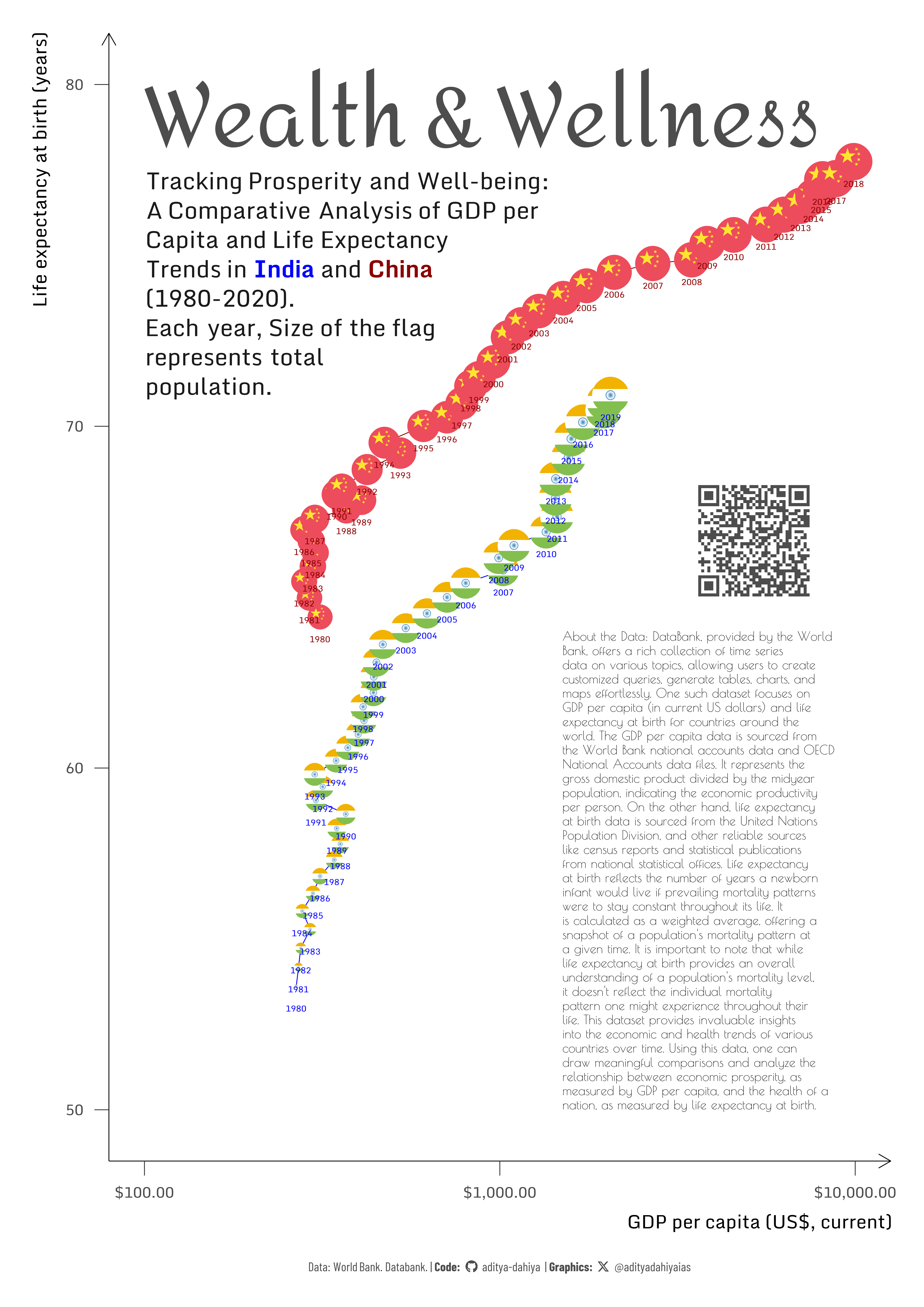
GDP per capita vs. Life Expectancy

I utilized data from the World Bank’s DataBank, a comprehensive analysis and visualization tool that houses a diverse collection of time series data spanning various topics. Specifically, I extracted information on Gross Domestic Product (GDP) and life expectancy for multiple countries over several years. Using this data, I created a scatter plot to explore the relationship between a country’s GDP and its life expectancy. The scatter plot allows for a visual examination of potential correlations or patterns between these two variables across different nations and over time. DataBank enables users to customize queries, generate tables, charts, and maps effortlessly, making it a valuable resource for data analysis and visualization. This tool facilitates not only the exploration of data but also the sharing and embedding of findings, encouraging collaboration and further analysis.

A time-series scatter-plot of India’s and China’s GDP-per-capita (on X-axis log scale) vs. Life expectancy at birth (on Y-axis), over time - each year is represented by a dot (flag) whose size corresponds to the total population that year.

How I made this graphic?

Loading required libraries, data import & creating custom functions

# Data Import and Wrangling Tools
library(tidyverse)            # All things tidy

# Final plot tools
library(scales)               # Nice Scales for ggplot2
library(fontawesome)          # Icons display in ggplot2
library(ggtext)               # Markdown text support for ggplot2
library(showtext)             # Display fonts in ggplot2
library(colorspace)           # Lighten and Darken colours
library(patchwork)            # Combining plots

# Extras and Annotations
library(magick)               # Image processing

# Credits: Geospatial Science and Human Security at ORNL
# Credits: @jpiburn, @petrbouchal, @bapfeld
# install.packages("wbstats")
library(wbstats)

# indicators <- wbstats::wb_indicators()

# indicators |> 
#   filter(str_detect(indicator_desc, "Life expectancy")) |> 
#   View()
# 
# indicators |> 
#   filter(str_detect(indicator_desc, "GDP per capita")) |> View()

# indicators |> 
#   filter(str_detect(indicator_id, "SP.POP.TOTL"))

selected_indicators <- c(
  "NY.GDP.PCAP.CD",
  "SP.POP.TOTL",
  "SP.DYN.LE00.IN"
)

rawdf <- wb_data(
  indicator = selected_indicators,
  start_date = 1980,
  end_date = 2023
  ) |>
  janitor::clean_names()

Exploratory Data Analysis & Data Wrangling

# rawdf |> visdat::vis_miss()

display_countries <- c("CN", "IN", "US", "ID", "MX", "NG", "PK")

df <- rawdf  |>
  rename(year = date) |> 
  complete(
    country, 
    year = 1980:2023, 
    fill = list(
      ny_gdp_pcap_cd = NA, 
      sp_dyn_le00_in = NA, 
      sp_pop_totl = NA
      )
    ) |> 
  tidyr::fill(
    ny_gdp_pcap_cd, 
    sp_dyn_le00_in, 
    sp_pop_totl,
    .direction = "updown"
    ) |> 
  mutate(
    ctry_label = if_else(
      iso2c %in% display_countries,
      country,
      NA
    )
  )

Visualization Parameters

# Font for titles
font_add_google("Poiret One",
  family = "title_font"
) 

font_add_google("Amita",
  family = "title2_font"
  )
# Font for the caption
font_add_google("Barlow Condensed",
  family = "caption_font"
) 

# Font for plot text
font_add_google("Monda",
  family = "body_font"
) 

ts <- 50

showtext_auto()

# Colour Palettes
mypal <- c("darkred", "blue")

bg_col <- "white"              # Background Colour
text_col <- "grey10"            # Colour for text
text_hil <- "grey30"            # Colour for highlighted text
 
# Caption stuff for the plot
sysfonts::font_add(
  family = "Font Awesome 6 Brands",
  regular = here::here("docs", "Font Awesome 6 Brands-Regular-400.otf")
)
github <- "&#xf09b"
github_username <- "aditya-dahiya"
xtwitter <- "&#xe61b"
xtwitter_username <- "@adityadahiyaias"
social_caption_1 <- glue::glue("<span style='font-family:\"Font Awesome 6 Brands\";'>{github};</span> <span style='color: {text_hil}'>{github_username}  </span>")
social_caption_2 <- glue::glue("<span style='font-family:\"Font Awesome 6 Brands\";'>{xtwitter};</span> <span style='color: {text_hil}'>{xtwitter_username}</span>")

Annotation Text for the Plot

plot_title <- "Wealth & Wellness"

plot_caption <- paste0(
  "Data: World Bank. Databank.", 
  " |  **Code:** ", 
  social_caption_1, 
  " |  **Graphics:** ", 
  social_caption_2
  )

plot_subtitle <- glue::glue("Tracking Prosperity and Well-being:<br>A Comparative Analysis of GDP per<br>Capita and\nLife Expectancy<br>Trends in <b style='color:{mypal[2]}'>India</b> and <b style='color:{mypal[1]}'>China</b><BR>(1980-2020).<br>Each year, Size of the flag<br>represents total<br>population.")

inset_text <- str_wrap("About the Data: DataBank, provided by the World Bank, offers a rich collection of time series data on various topics, allowing users to create customized queries, generate tables, charts, and maps effortlessly. One such dataset focuses on GDP per capita (in current US dollars) and life expectancy at birth for countries around the world. The GDP per capita data is sourced from the World Bank national accounts data and OECD National Accounts data files. It represents the gross domestic product divided by the midyear population, indicating the economic productivity per person. On the other hand, life expectancy at birth data is sourced from the United Nations Population Division, and other reliable sources like census reports and statistical publications from national statistical offices. Life expectancy at birth reflects the number of years a newborn infant would live if prevailing mortality patterns were to stay constant throughout its life. It is calculated as a weighted average, offering a snapshot of a population's mortality pattern at a given time. It is important to note that while life expectancy at birth provides an overall understanding of a population's mortality level, it doesn't reflect the individual mortality pattern one might experience throughout their life. This dataset provides invaluable insights into the economic and health trends of various countries over time. Using this data, one can draw meaningful comparisons and analyze the relationship between economic prosperity, as measured by GDP per capita, and the health of a nation, as measured by life expectancy at birth.", 50, whitespace_only = FALSE)

An animated plot

library(gganimate)

g <- df |> 
  arrange(desc(sp_pop_totl)) |> 
  ggplot(
    aes(
      x = ny_gdp_pcap_cd,
      y = sp_dyn_le00_in,
      size = sp_pop_totl,
      label = ctry_label
    )
  ) +
  geom_point(
    fill = "orange",
    alpha = 0.5,
    shape = 21
  ) +
  scale_size(
    range = c(1, 10)
  ) +
  scale_x_continuous(
    labels = scales::label_currency(),
    transform = "log2",
    breaks = c(1000, 10000, 100000)
  ) +
  scale_y_continuous(
    limits = c(40, 90)
  ) +
  geom_text(
    size = 3,
    check_overlap = TRUE
    ) +
  labs(
    title = "Year: {frame_time}",
    subtitle = "Rising life expectancies with rising wealth for countries",
    x = "GDP per capita (US Dollars, current)",
    y = "Life expectancy at birth (years)"
  ) +
  theme_classic(
    base_family = "body_font",
    base_size = 12
  ) +
  theme(
    legend.position = "none",
    panel.grid = element_line(
      colour = "lightgrey",
      linetype = 3,
      linewidth = 0.5
    ),
    axis.line = element_line(
      arrow = arrow()
    )
  ) +
  transition_time(as.integer(year)) +
  ease_aes("linear")


# Animate the plot
animate(
  plot = g,
  fps = 5,
  height = 500,
  width = 400,
  end_pause = 20
)

The base plot

g_base <- df |>
  filter(iso2c %in% c("IN", "CN")) |> 
  mutate(iso2c = str_to_lower(iso2c)) |> 
  filter(year <= 2019) |> 
  ggplot(
    aes(
      x = ny_gdp_pcap_cd, 
      y = sp_dyn_le00_in,
      colour = country
    )
  ) +
  geom_path() +
  ggflags::geom_flag(
    aes(
      country = iso2c,
      size = sp_pop_totl
    )
  ) +
  geom_text(
    aes(
      label = year
    ),
    nudge_y = -0.65,
    size = 12,
    family = "body_font"
  ) +
  scale_x_continuous(
    trans = "log2",
    breaks = c(100, 1000, 10000),
    labels = scales::label_currency(),
    limits = c(100, 10000)
  ) +
  scale_y_continuous(
    limits = c(50, 80)
  ) +
  scale_size(
    range = c(2, 20)
  ) +
  scale_colour_manual(
    values = mypal[1:2]
  ) +
  labs(
    x = "GDP per capita (US$, current)",
    y = "Life expectancy at birth (years)",
    caption = plot_caption
  ) +
  annotate(
    geom = "text",
    x = 100, y = 80,
    label = plot_title,
    hjust = 0,
    vjust = 1,
    family = "title2_font",
    size = 2.4 * ts,
    colour = text_hil
  ) +
  annotate(
    geom = "richtext",
    x = 100, y = 77.5,
    label = plot_subtitle,
    hjust = 0,
    vjust = 1,
    family = "body_font",
    size = ts/1.5,
    colour = text_col,
    fill = "transparent",
    label.size = 0,
    lineheight = 0.4
  ) +
  annotate(
    geom = "text",
    x = 1500,
    y = 64,
    hjust = 0, 
    vjust = 1,
    label = inset_text,
    family = "title_font",
    colour = text_col,
    size = ts/2.8,
    lineheight = 0.3
  ) +
  theme_classic(
    base_size = 1.5 * ts,
    base_family = "body_font"
  ) +
  theme(
    legend.position = "none",
    plot.title.position = "plot",
    axis.line = element_line(
      arrow = arrow(),
      linewidth = 0.5
    ),
    axis.ticks = element_line(
      linewidth = 0.5
    ),
    axis.title = element_text(hjust = 1),
    plot.caption = element_textbox(
      family = "caption_font",
      hjust = 0.5,
      size = ts,
      colour = text_hil
    )
  )

Adding annotations to the plot

# A QR Code for the infographic
url_graphics <- paste0(
  "https://aditya-dahiya.github.io/projects_presentations/data_vizs/",
  # The file name of the current .qmd file
  "wb_gdp_lifeexp",         
  ".html"
)
# remotes::install_github('coolbutuseless/ggqr')
# library(ggqr)
plot_qr <- ggplot(
  data = NULL, 
  aes(x = 0, y = 0, label = url_graphics)
  ) + 
  ggqr::geom_qr(
    colour = text_hil, 
    fill = bg_col,
    size = 2
    ) +
  coord_fixed() +
  theme_void() +
  theme(plot.background = element_rect(
    fill = NA, 
    colour = NA
    ),
    panel.background = element_rect(
      fill = NA,
      colour = NA
    )
  )

# Compiling the plots

g <- g_base +
  inset_element(
    p = plot_qr,
    left = 0.75, right = 0.90,
    bottom = 0.5, top = 0.6,
    align_to = "panel",
    clip = FALSE
  ) + 
  plot_annotation(
    theme = theme(
      plot.background = element_rect(
        fill = "transparent",
        colour = "transparent"
      )
    )
  )

Savings the graphics

ggsave(
  filename = here::here("data_vizs", "a4_wb_gdp_lifeexp.png"),
  plot = g,
  width = 2 * 210,        
  height = 2 * 297,   
  units = "mm",
  bg = "white"
)


# Saving a thumbnail for the webpage
image_read(here::here("data_vizs", "a4_wb_gdp_lifeexp.png")) |> 
  image_resize(geometry = "400") |> 
  image_write(here::here("data_vizs", 
                         "thumbnails", 
                         "wb_gdp_lifeexp.png"))