The Coastal Gravity: Where Humanity Chooses to Live

Combining {terra}, {tidyterra}, {geodata}, {ggtext}, and {patchwork} to analyze 33 years of global population distribution across elevation bands.

World Bank Data

A4 Size Viz

Governance

Demographics

Public Health

Geocomputation

Raster

{terra}

{geodata}

Author

Aditya Dahiya

Published

November 3, 2025

About the Data

The GlobPOP dataset (GlobPOP GitHub Repository) is a comprehensive 33-year (1990-2022) global gridded population product generated through cluster analysis and statistical learning. The data, which has a spatial resolution of 30 arcseconds (approximately 1km), is provided in GeoTIFF format for easy integration and analysis, featuring two key population formats: ‘Count’ and ‘Density’. The primary, continuous GlobPOP 1990-2022 dataset can be freely accessed on Zenodo (Zenodo Data Access). Researchers can find the methodology and initial scope (1990-2020) detailed in the corresponding article published in Scientific Data (Sci Data 11, 124 (2024)). For a visual and comparative understanding of the data’s temporal accuracy, an interactive web application (GlobPOP ShinyApp) for time-series analysis is also available. Specific citation links are provided for the methodology Code (Code Citation on Zenodo) and the Updated Dataset version 3.0 (Updated Dataset Citation on Zenodo).

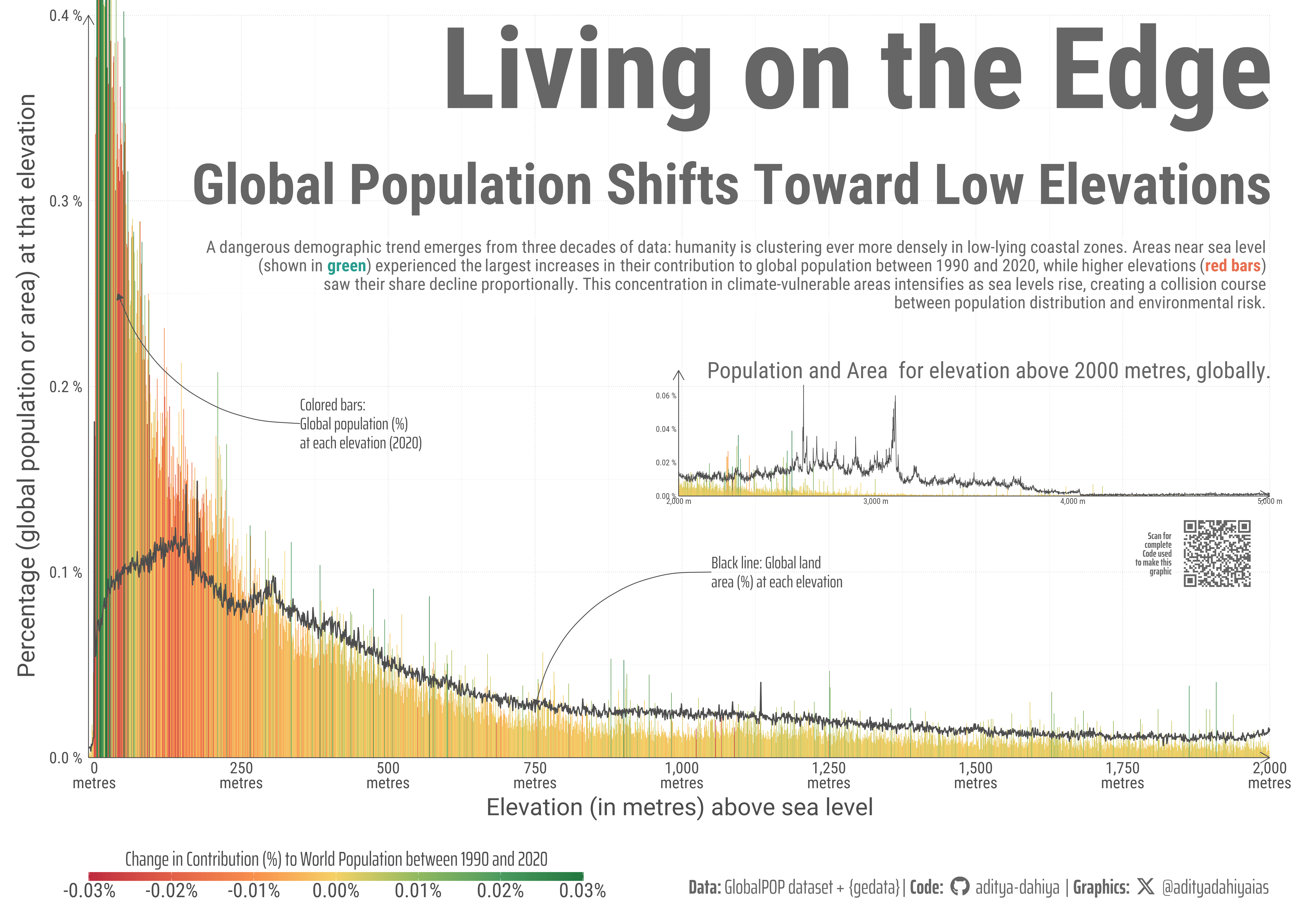
This chart compares global population distribution with Earth’s topography across elevation bands. The black line represents the percentage of Earth’s surface area at each elevation above sea level. Colored vertical bars show the percentage of world population living at each elevation in 2020, with bar colors indicating change from 1990 to 2020: green shows elevation bands where population share increased, red where it decreased. Bar height reflects concentration—taller bars indicate more people living at that elevation relative to available land area.

How I made this graphic?

Loading required libraries, data import & creating custom functions

Code

# Data Import and Wrangling Tools
pacman::p_load(
  tidyverse,    # Data Wrangling and Plotting
  scales,       # Nice scales for ggplot2
  fontawesome,  # Icons display in ggplot2
  ggtext,       # Markdown text support ggplot2
  showtext,     # Display fonts in ggplot2
  colorspace,   # Lighten and darken colours
  patchwork,    # Combining plots together
  magick,       # Image processing and editing
  terra,        # Handling Rasters in R
  tidyterra,    # Plotting Rasters with ggplot2
  sf,           # Handling geometric objects
  geodata       # Get elevation data
)

Visualization Parameters

Code

# Font for titles
font_add_google("Roboto",
  family = "title_font"
) 

# Font for the caption
font_add_google("Saira Extra Condensed",
  family = "caption_font"
) 

# Font for plot text
font_add_google("Roboto Condensed",
  family = "body_font"
) 

showtext_auto()

# A base Colour
bg_col <- "white"
seecolor::print_color(bg_col)

# Colour for highlighted text
text_hil <- "grey40"
seecolor::print_color(text_hil)

# Colour for the text
text_col <- "grey30"
seecolor::print_color(text_col)

line_col <- "grey30"

# Define Base Text Size
bts <- 80

mypal1 <- paletteer::paletteer_d("rcartocolor::SunsetDark")
mypal2 <- paletteer::paletteer_d("rcartocolor::ag_GrnYl", direction = -1)


# Caption stuff for the plot
sysfonts::font_add(
  family = "Font Awesome 6 Brands",
  regular = here::here("docs", "Font Awesome 6 Brands-Regular-400.otf")
)
github <- "&#xf09b"
github_username <- "aditya-dahiya"
xtwitter <- "&#xe61b"
xtwitter_username <- "@adityadahiyaias"
social_caption_1 <- glue::glue("<span style='font-family:\"Font Awesome 6 Brands\";'>{github};</span> <span style='color: {text_hil}'>{github_username}  </span>")
social_caption_2 <- glue::glue("<span style='font-family:\"Font Awesome 6 Brands\";'>{xtwitter};</span> <span style='color: {text_hil}'>{xtwitter_username}</span>")
plot_caption <- paste0(
  "**Data:**  GlobalPOP dataset + {gedata}",
  " |  **Code:** ",
  social_caption_1,
  " |  **Graphics:** ",
  social_caption_2
)
rm(
  github, github_username, xtwitter,
  xtwitter_username, social_caption_1,
  social_caption_2
)

Annotation Text for the Plot

Code

plot_title1 <- "Living on the Edge"

plot_title2 <- "Global Population Shifts Toward Low Elevations"

plot_subtitle <- "A dangerous demographic trend emerges from three decades of data: humanity is clustering ever more densely in low-lying coastal zones. Areas near sea level<br>(shown in <span style='color:#2a9d8f;'>**green**</span>) experienced the largest increases in their contribution to global population between 1990 and 2020, while higher elevations (<span style='color:#e76f51;'>**red bars**</span>)<br>saw their share decline proportionally. This concentration in climate-vulnerable areas intensifies as sea levels rise, creating a collision course<br>between population distribution and environmental risk."
str_view(plot_subtitle)

inset_text <- "world_elev_pop_chart"

str_view(inset_text, pattern = "<br>")

Loading of temporarily saved files.

Code

# ----------------------------------------------------------------------
# SAVE ELEVATION DATA AND RASTER
# ----------------------------------------------------------------------

# # Save the elevation data tibbles as RDS files (preserves R data structure)
# saveRDS(
#   all_elev_data, 
#   file = "all_elev_data.rds"
# )
# 
# saveRDS(
#   all_elev_data_summary, 
#   file = "all_elev_data_summary.rds"
# )
# 
# saveRDS(
#   elev_area_summary,
#   file = "elevation_area_summary.rds"
# )
# # Save the elevation raster (terra format)
# terra::writeRaster(
#   elev_raster,
#   filename = "elev_raster.tif",
#   overwrite = TRUE
# )

# Save the resampled elevation raster (matched to population data)
# terra::writeRaster(
#   elev_resampled,
#   filename = "elev_resampled.tif",
#   overwrite = TRUE
# )

# ----------------------------------------------------------------------
# TO LOAD THESE FILES LATER
# ----------------------------------------------------------------------

# To load the data in a new session:
all_elev_data <- readRDS("all_elev_data.rds")
elev_area_summary <- readRDS("elevation_area_summary.rds")
all_elev_data_summary <- readRDS("all_elev_data_summary.rds")
elev_raster <- terra::rast("elev_raster.tif")
# elev_resampled <- terra::rast("elev_resampled.tif")

Getting World Elevation Raster using `{geodata}`

Code

# 1. Define the directory where the data will be downloaded/stored.
# We use tempdir() to ensure the file is saved temporarily, but you can
# replace this with a permanent path if you plan to reuse the data.
data_path <- tempdir()

# 2. Download the global elevation raster (ETOPO1 data source)
elev_raster <- geodata::elevation_global(
  res = 0.5,
  path = data_path
)

# 3. Print the result to confirm it contains elevation values (in meters)
# print(elev_raster)

# 4. (Optional) Basic plot to visualize the global elevation
# The values are in meters, showing land elevation and ocean bathymetry.
# 
# plot(
#   elev_raster, main = "World Elevation Raster (ETOPO1, 30 arc-sec resolution)"
#   )

# Reduce resolution significantly (aggregate by factor of 10-20)
# Compute the percentage area of world for each elevation level
elev_area_summary <- elev_raster |>
  aggregate(fact = 20, fun = "mean") |>  # Reduces resolution 20x
  round() |>
  freq(bylayer = TRUE) |>
  as_tibble() |>
  filter(!is.na(value)) |>
  mutate(
    elevation_m = as.integer(value),
    total_area_m2 = count * {
      elev_raster |>
        aggregate(fact = 20, fun = "mean") |>
        cellSize(unit = "m") |>
        values(na.rm = TRUE) |>
        mean()
    }
  ) |>
  mutate(pct_world_area = (total_area_m2 / sum(total_area_m2)) * 100) |>
  select(elevation_m, pct_world_area, count, total_area_m2) |>
  arrange(elevation_m)

# View results
# elev_area_summary

Getting Population Raster Data and Analysis

Code

# ----------------------------------------------------------------------
# FUNCTION TO ANALYZE POPULATION BY ELEVATION FOR A GIVEN YEAR
# ----------------------------------------------------------------------

#' Analyzes population distribution by 1-meter elevation bands for a given year
#'
#' @param year Integer representing the year (e.g., 1990)
#' @param elev_raster Terra SpatRaster of elevation data
#' @return A tibble with elevation bands and population percentages
analyze_pop_by_elevation <- function(year, elev_raster) {
  
  # 2.1 Load population raster for the year
  filename <- paste0("GlobPOP_Count_30arc_", year, "_I32.tiff")
  message("Processing year: ", year, " (File: ", filename, ")")
  
  if (!file.exists(filename)) {
    warning("File not found for year ", year, ": ", filename, ". Skipping.")
    return(NULL)
  }
  
  # Load and aggregate population raster
  pop_raster <- terra::rast(filename) |>
    terra::aggregate(fact = 10)
  
  # 2.2 Resample elevation to match population raster resolution and extent
  elev_resampled <- terra::resample(
    elev_raster, 
    pop_raster, 
    method = "bilinear"
  )
  
  # 2.3 Convert both rasters to data frames
  pop_col_name <- names(pop_raster)
  
  # Combine elevation and population data
  combined_data <- terra::as.data.frame(
    c(elev_resampled, pop_raster),
    xy = TRUE,
    na.rm = TRUE
  ) |>
    dplyr::as_tibble()
  
  # Rename columns for clarity
  elev_col_name <- names(elev_resampled)
  combined_data <- combined_data |>
    dplyr::rename(
      elevation = !!elev_col_name,
      population = !!pop_col_name
    )
  
  # 2.4 Calculate total global population
  total_global_pop <- sum(combined_data$population, na.rm = TRUE)
  
  # 2.5 Create 1-meter elevation bands
  pop_by_elevation <- combined_data |>
    # Round elevation to nearest meter (e.g., 1m represents 0.5 to 1.5m)
    dplyr::mutate(elevation_band = round(elevation)) |>
    # Group by elevation band
    dplyr::group_by(elevation_band) |>
    # Sum population for each band
    dplyr::summarise(
      pop_in_band = sum(population, na.rm = TRUE),
      .groups = "drop"
    ) |>
    # Calculate percentage relative to total global population
    dplyr::mutate(
      percent_global_pop = (pop_in_band / total_global_pop) * 100,
      year = as.factor(year)
    ) |>
    # Rename for clarity
    dplyr::rename(elevation_m = elevation_band)
  
  return(pop_by_elevation)
}

# ----------------------------------------------------------------------
# 3. ANALYZE ALL YEARS (1990-2020)
# ----------------------------------------------------------------------

# Define years to analyze
years_to_analyze <- seq(1990, 2020, 5)

# Apply the function to all years
all_elevation_results <- purrr::map(
  years_to_analyze, 
  ~analyze_pop_by_elevation(.x, elev_raster)
) |>
  purrr::compact() # Remove NULL entries if any files were missing

# Combine all years into a single tibble
all_elev_data <- dplyr::bind_rows(all_elevation_results)

# ----------------------------------------------------------------------
# 4. CREATE SUMMARY FOR 1990 vs 2020 COMPARISON
# ----------------------------------------------------------------------

all_elev_data_summary <- all_elev_data |>
  # Ensure year is numeric for easy filtering
  dplyr::mutate(year_num = as.numeric(as.character(year))) |>
  # Filter for start (1990) and end (2020) years
  dplyr::filter(year_num %in% c(1990, 2020)) |>
  # Select key columns
  dplyr::select(elevation_m, year_num, percent_global_pop) |>
  # Pivot wider to compare 1990 and 2020 side-by-side
  tidyr::pivot_wider(
    names_from = year_num,
    values_from = percent_global_pop,
    names_prefix = "pop_pct_",
    values_fill = 0  # Fill missing elevations with 0
  ) |>
  # Calculate change metrics
  dplyr::mutate(
    # Absolute change in percentage contribution
    change_contribution_absolute = pop_pct_2020 - pop_pct_1990,
    # Relative change in percentage contribution
    change_contribution = dplyr::case_when(
      pop_pct_1990 == 0 ~ NA_real_,
      TRUE ~ ((pop_pct_2020 - pop_pct_1990) / pop_pct_1990) * 100
    )
  ) |>
  # Add current population percentage for plotting
  left_join(
    all_elev_data |>
      filter(year == "2020") |>
      select(elevation_m, percent_global_pop),
    by = "elevation_m"
  )

Make an inset chart for elevation above 2000 metres

Code

g_inset <- ggplot() +
  geom_col(
    data = all_elev_data_summary,
    mapping = aes(
      x = elevation_m,
      y = pop_pct_2020,
      colour = change_contribution_absolute,
      fill = change_contribution_absolute
    ),
    width = 0.1,
    linewidth = 0.3,
    alpha = 0.5
  ) +
  geom_line(
    data = elev_area_summary,
    mapping = aes(
      x = elevation_m,
      y = pct_world_area
    ),
    linewidth = 0.35,
    colour = text_col
  ) +
  annotate(
    geom = "text",
    x = 5000,
    y = 0.08,
    label = "Population and Area  for elevation above 2000 metres, globally.",
    hjust = 1,
    vjust = 1,
    family = "body_font",
    size = bts / 2.5,  
    colour = text_hil,
    lineheight = 0.25
  ) +
  scale_x_continuous(
    limits = c(2000, 5000),
    label = label_number(suffix = " m", big.mark = ",")
  ) +
  scale_y_continuous(
    label = label_number(suffix = " %")
  ) +
  coord_cartesian(
    ylim = c(0, 0.075),
    clip = "off",
    expand = FALSE
  ) +
  paletteer::scale_fill_paletteer_c(
    "ggthemes::Red-Green-Gold Diverging",
    limits = c(-0.02, 0.02),,
    oob = scales::squish,
    name = NULL,
    labels = label_number(suffix = "%")
  ) +
  paletteer::scale_colour_paletteer_c(
    "ggthemes::Red-Green-Gold Diverging",
    limits = c(-0.02, 0.02),,
    oob = scales::squish,
    name = NULL,
    labels = label_number(suffix = "%")
  ) +
  labs(
    title = NULL,
    subtitle = NULL,
    caption = NULL,
    x = NULL,
    y = NULL
  ) +
  theme_minimal(
    base_size = bts / 2,
    base_family = "body_font"
  ) +
  theme(
    # Overall
    text = element_text(
      margin = margin(0,0,0,0, "mm"),
      colour = text_col,
      lineheight = 0.3
    ),
    legend.position = "none",
    
    # Axes
    axis.line.y.left = element_line(
      linewidth = 0.5,
      colour = text_col,
      arrow = arrow(
        length = unit(5, "mm")
      )
    ),
    axis.line.x.bottom = element_line(
      arrow = arrow(
        length = unit(5, "mm")
      ),
      linewidth = 0.5,
      colour = text_col
    ),
    axis.text.x.bottom = element_text(
      margin = margin(1,1,1,1, "mm"),
      lineheight = 0.25
    ),
    axis.text.y.left = element_text(
      margin = margin(1,1,1,1, "mm")
    ),
    axis.title.y.left = element_text(
      margin = margin(0,0,0,0, "mm")
    ),
    axis.title.x.bottom = element_text(
      margin = margin(0,0,0,0, "mm")
    ),
    axis.title.x.top = element_text(
      margin = margin(0,0,0,0, "mm")
    ),
    
    # Panel and Legend
    panel.grid = element_blank(),
    plot.margin = margin(0,15,0,0, "mm"),
    panel.background = element_rect(
      fill = NA,
      colour = NA
    ),
    plot.background = element_rect(
      fill = NA,
      colour = NA
    )
  )

The Base Plot

Code

g <- ggplot() +
  geom_col(
    data = all_elev_data_summary,
    mapping = aes(
      x = elevation_m,
      y = pop_pct_2020,
      colour = change_contribution_absolute,
      fill = change_contribution_absolute
    ),
    width = 0.1,
    linewidth = 0.3,
    alpha = 0.5
  ) +

  geom_line(
    data = elev_area_summary,
    mapping = aes(
      x = elevation_m,
      y = pct_world_area
    ),
    linewidth = 0.75,
    colour = text_col
  ) +

  # Add plot title annotation
  annotate(
    geom = "text",
    x = 2000,
    y = 0.35,
    label = plot_title1,
    hjust = 1,
    vjust = 0,
    family = "body_font",
    size = bts * 2 ,  
    colour = text_hil,
    fontface = "bold",
    lineheight = 0.25
  ) +
  annotate(
    geom = "text",
    x = 2000,
    y = 0.32,
    label = plot_title2,
    hjust = 1,
    vjust = 1,
    family = "body_font",
    size = bts ,  
    colour = text_hil,
    fontface = "bold",
    lineheight = 0.25
  ) +
  # Add plot subtitle annotation
  annotate(
    geom = "richtext",
    x = 2000,
    y = 0.28,  # Slightly below title
    label = plot_subtitle,
    hjust = 1,
    vjust = 1,
    family = "body_font",
    size = 0.3 * bts,  
    colour = text_hil,
    lineheight = 0.35,
    fill = alpha(bg_col, 0.5),
    label.color = NA
  ) +
  
  # Annotation for the global land area black line
  geom_curve(
    aes(x = 1050, y = 0.1, xend = 750, yend = 0.028),
    arrow = arrow(length = unit(3, "mm"), type = "closed"),
    curvature = 0.4,
    linewidth = 0.5,
    colour = text_col
  ) +
  annotate(
    geom = "text",
    x = 1050,
    y = 0.1,
    label = "Black line: Global land\narea (%) at each elevation",
    hjust = 0,
    vjust = 0.5,
    family = "caption_font",
    size = 0.3 * bts,
    colour = text_col,
    lineheight = 0.3
  ) +
  
  # Annotation for BARS (population) - pointing to prominent bars near sea level
  geom_curve(
    aes(x = 350, y = 0.18, xend = 40, yend = 0.25),
    arrow = arrow(length = unit(3, "mm"), type = "closed"),
    curvature = -0.35,
    linewidth = 0.5,
    colour = text_col
  ) +
  annotate(
    geom = "text",
    x = 350,
    y = 0.18,
    label = "Colored bars:\nGlobal population (%)\nat each elevation (2020)",
    hjust = 0,
    vjust = 0.5,
    family = "caption_font",
    size = 0.3 * bts,
    colour = text_col,
    lineheight = 0.3
  ) +
    
  scale_x_continuous(
    limits = c(-10, 2000),
    breaks = seq(0, 2000, 250),
    label = label_number(suffix = "\nmetres", big.mark = ",")
  ) +
  scale_y_continuous(
    label = label_number(suffix = " %")
  ) +
  coord_cartesian(
    ylim = c(0, 0.4),
    clip = "off",
    expand = FALSE
  ) +
  paletteer::scale_fill_paletteer_c(
    "ggthemes::Red-Green-Gold Diverging",
    limits = c(-0.03, 0.03),,
    oob = scales::squish,
    name = "Change in Contribution (%) to World Population between 1990 and 2020",
    labels = label_number(suffix = "%")
  ) +
  paletteer::scale_colour_paletteer_c(
    "ggthemes::Red-Green-Gold Diverging",
    limits = c(-0.03, 0.03),,
    oob = scales::squish,
    name = "Change in Contribution (%) to World Population between 1990 and 2020",
    labels = label_number(suffix = "%")
  ) +
  labs(
    title = NULL,
    subtitle = NULL,
    caption = plot_caption,
    x = "Elevation (in metres) above sea level",
    y = "Percentage (global population or area) at that elevation"
  ) +
  theme_minimal(
    base_size = bts,
    base_family = "body_font"
  ) +
  theme(
    # Overall
    text = element_text(
      margin = margin(0,0,0,0, "mm"),
      colour = text_col,
      lineheight = 0.3
    ),
    
    # Axes
    axis.line.y.left = element_line(
      arrow = arrow(
        length = unit(5, "mm")
      ),
      linewidth = 0.5,
      colour = text_col
    ),
    axis.line.x.bottom = element_line(
      arrow = arrow(
        length = unit(5, "mm")
      ),
      linewidth = 0.5,
      colour = text_col
    ),
    axis.text.x.bottom = element_text(
      margin = margin(2,2,2,2, "mm"),
      lineheight = 0.25
    ),
    axis.text.y.left = element_text(
      margin = margin(3,3,3,3, "mm")
    ),
    axis.title.y.left = element_text(
      family = "title_font",
      size = 1.2 * bts,
      margin = margin(1,1,1,1, "mm")
    ),
    axis.title.x.bottom = element_text(
      family = "title_font",
      size = 1.2 * bts,
      margin = margin(1,1,1,1, "mm")
    ),
    axis.title.x.top = element_text(
      margin = margin(1,1,1,1, "mm")
    ),
    
    plot.title = element_text(
        margin = margin(5, 0, 5, 0, "mm"),
        hjust = 0.5,
        vjust = 0.5,
        colour = text_hil,
        size = 2 * bts,
        family = "body_font",
        face = "bold",
        lineheight = 0.25
      ),
    plot.subtitle = element_text(
        margin = margin(5,0,5,0, "mm"),
        hjust = 0,
        lineheight = 0.3,
        size = 0.85 * bts,
        family = "body_font",
        colour = text_hil
      ),
    plot.caption = element_markdown(
        family = "caption_font",
        margin = margin(25,0,5,0, "mm"),
        colour = text_hil,
        size = bts,
        hjust = 1
      ),
    
    # Panel and Legend
    panel.grid = element_line(
      linewidth = 0.3,
      colour = alpha("grey70", 1),
      linetype = 3
    ),
    legend.position = "inside",
    legend.position.inside = c(0, 0),
    legend.direction = "horizontal",
    legend.justification = c(0, 1),
    legend.margin = margin(40,0,0,0, "mm"),
    legend.box.margin = margin(0,0,0,0, "mm"),
    legend.key.width = unit(45, "mm"),
    legend.key.height = unit(4, "mm"),
    legend.title.position = "top",
    legend.text = element_text(
      margin = margin(1,0,0,0, "mm"),
      size = bts
    ),
    legend.title = element_text(
      margin = margin(2,0,2,0, "mm"),
      size = bts,
      hjust = 0.5,
      family = "caption_font"
    ),
    plot.margin = margin(5,15,5,5, "mm")
  )

Adding QR code to the plot

Code

# A QR Code for the infographic
url_graphics <- paste0(
  "https://aditya-dahiya.github.io/projects_presentations/data_vizs/",
  # The file name of the current .qmd file
  "world_elev_pop_chart",         
  ".html"
)
# remotes::install_github('coolbutuseless/ggqr')
# library(ggqr)
plot_qr <- ggplot(
  data = NULL, 
  aes(x = 0, y = 0, label = url_graphics)
  ) + 
  ggqr::geom_qr(
    colour = text_hil, 
    fill = bg_col,
    size = 1.2
    ) +
  annotate(
    geom = "text",
    x = -0.05,
    y = 0,
    label = "Scan for complete Code used to make this graphic" |> str_wrap(12),
    hjust = 1,
    vjust = 0.5,
    family = "caption_font",
    colour = text_hil,
    size = bts / 6,
    lineheight = 0.25,
    fontface = "bold"
  ) +
  coord_fixed(clip = "off") +
  theme_void() +
  theme(
    plot.background = element_rect(
      fill = NA, 
      colour = NA
    ),
    panel.background = element_rect(
      fill = NA,
      colour = NA
    ),
    plot.margin = margin(0, 10, 0, 0, "mm")
  )

Combining the Plots

Code

g_full <- g +
  inset_element(
    p = g_inset,
    left = 0.5, right = 1,
    top = 0.6, bottom = 0.45,
    align_to = "full",
    clip = FALSE
  ) +
  inset_element(
    p = plot_qr,
    left = 0.85, right = 1,
    top = 0.45, bottom = 0.35,
    align_to = "full",
    clip = FALSE
  )

ggsave(
  filename = here::here(
    "data_vizs",
    "a4_world_elev_pop_chart.png"
  ),
  plot = g_full,
  width = 297 * 2,
  height = 210 * 2,
  units = "mm",
  bg = bg_col
)

Savings the graphics

Code

# Saving a thumbnail for the webpage
image_read(here::here("data_vizs", "a4_world_elev_pop_chart.png")) |> 
  image_resize(geometry = "400") |> 
  image_write(here::here("data_vizs", 
                         "thumbnails", 
                         "world_elev_pop_chart.png"))

Session Info

Code

# Data Import and Wrangling Tools
pacman::p_load(
  tidyverse,    # Data Wrangling and Plotting
  scales,       # Nice scales for ggplot2
  fontawesome,  # Icons display in ggplot2
  ggtext,       # Markdown text support ggplot2
  showtext,     # Display fonts in ggplot2
  colorspace,   # Lighten and darken colours
  patchwork,    # Combining plots together
  magick,       # Image processing and editing
  terra,        # Handling Rasters in R
  tidyterra,    # Plotting Rasters with ggplot2
  sf            # Handling geometric objects
)

sessioninfo::session_info()$packages |>
  as_tibble() |>
  
  # The attached column is TRUE for packages that were 
  # explicitly loaded with library()
  dplyr::filter(attached == TRUE) |>
  dplyr::select(package,
    version = loadedversion,
    date, source
  ) |>
  dplyr::arrange(package) |>
  janitor::clean_names(
    case = "title"
  ) |>
  gt::gt() |>
  gt::opt_interactive(
    use_search = TRUE
  ) |>
  gtExtras::gt_theme_espn()

Table 1: R Packages and their versions used in the creation of this page and graphics

About the Data

How I made this graphic?

Loading required libraries, data import & creating custom functions

Visualization Parameters

Annotation Text for the Plot

Getting World Elevation Raster using {geodata}

Getting Population Raster Data and Analysis

Make an inset chart for elevation above 2000 metres

The Base Plot

Adding QR code to the plot

Combining the Plots

Savings the graphics

Session Info

Getting World Elevation Raster using `{geodata}`