Geocomputation for race elevation profiles: Mapping the UTMB Ultramarathon
This analysis leverages spatial packages like sf, terra, and tidyterra for data manipulation, while ggplot2 and ggblend enhance visualization. Techniques include raster blending, hillshade creation with whitebox, and custom theming for a detailed, informative map of the UTMB ultramarathon route.
Maps
{ggblend}
{whitebox}
{osmdata}
{elevatr}
Geocomputation
Elevation Profile
Hill Shade
Author
Aditya Dahiya
Published
April 14, 2025
About the UTMB Mont Blanc Ultra-Marathon
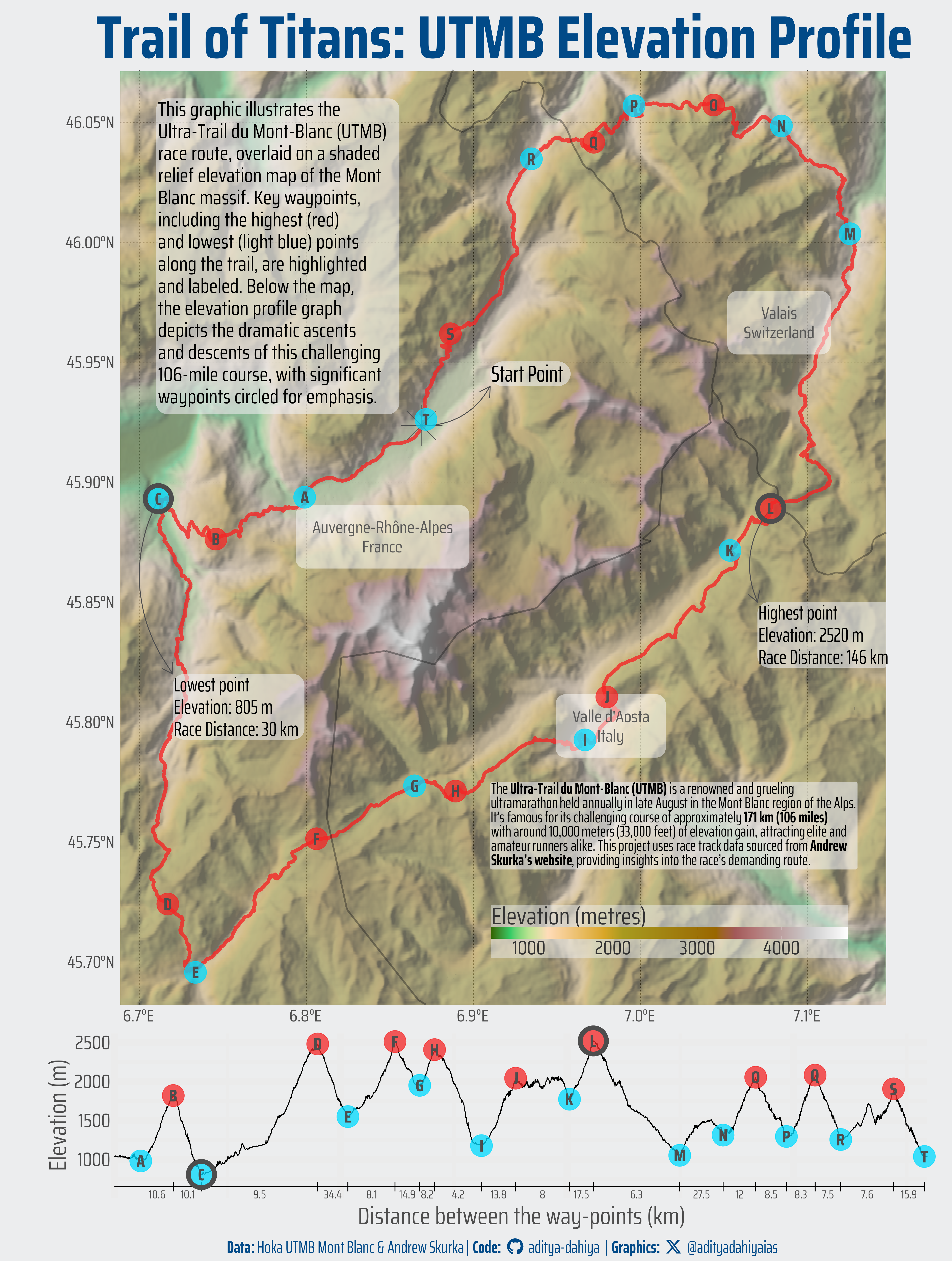
The Ultra-Trail du Mont-Blanc (UTMB) is an iconic and challenging ultramarathon that takes place annually in the Alps, crossing through France, Italy, and Switzerland. Covering approximately 176 kilometers with around 10,000 meters of elevation gain, it’s known as the “most mythical and prestigious trail running race in the world” (UTMB). Created in 2003, the UTMB has become the 100M final of the UTMB World Series, attracting both elite and amateur runners who share the same extraordinary course. While the exact route may vary slightly each year (this current data is sourced from Andrew Skurka, 2017), the race offers an introspective adventure amidst stunning landscapes, pushing participants to their limits as they strive to cross the finish line in Chamonix.
Figure 1: This graphic visualizes the UTMB ultramarathon route on a shaded relief map with key waypoints highlighted. The elevation profile shows dramatic ascents and descents. Created using {sf}, {tidyverse}, {leaflet}, {mapview}, and {patchwork} for spatial analysis and visualization.
Load packages
Code
# Spatial data handling and plottinglibrary(sf) # Import, export, and manipulate vector datalibrary(terra) # Import, export, and manipulate raster datalibrary(tidyterra) # Helper functions for using terra with ggplot2# Data wrangling & visualizationlibrary(tidyverse) # Data manipulation & visualizationlibrary(magrittr) # Writing Code in pipes# Getting additional datalibrary(osmdata) # Getting Open Street Maps datalibrary(geodata) # Countries and Counties Mapslibrary(elevatr) # Elevation Data# Interactive Visualizationlibrary(mapview) # Interactive Mapslibrary(leaflet) # Extensions to mapviewlibrary(leafpop) # Pop-up customization# Final plot toolslibrary(scales) # Nice Scales for ggplot2library(fontawesome) # Icons display in ggplot2library(ggtext) # Markdown text in ggplot2library(showtext) # Display fonts in ggplot2library(patchwork) # Composing Plots
Getting data
Code
# URL from Andrew Skurka's website # Read the downloaded GPX fileutmb_route <- sf::read_sf("https://www.dropbox.com/s/uqertaurpu4d1x2/UTMB-Course-GPX.gpx?dl=1",layer ="tracks" ) |>st_transform("EPSG:4326")
Visualization Parameters
Code
# Font for titlesfont_add_google("Saira",family ="title_font") # Font for the captionfont_add_google("Saira Extra Condensed",family ="caption_font") # Font for plot textfont_add_google("Saira Condensed",family ="body_font") showtext_auto()# Palette extracted from https://montblanc.utmb.world/races/UTMBmypal <-c("#F42525", "#00DBFF", "#111A2E", "#014A88", "#ECEDEE","#FFFFFF" )# A base Colourbg_col <- mypal[5]seecolor::print_color(bg_col)# Colour for highlighted texttext_hil <- mypal[4]seecolor::print_color(text_hil)# Colour for the texttext_col <-"grey30"seecolor::print_color(text_col)# Define Base Text Sizebts <-90# Caption stuff for the plotsysfonts::font_add(family ="Font Awesome 6 Brands",regular = here::here("docs", "Font Awesome 6 Brands-Regular-400.otf"))github <-""github_username <-"aditya-dahiya"xtwitter <-""xtwitter_username <-"@adityadahiyaias"social_caption_1 <- glue::glue("<span style='font-family:\"Font Awesome 6 Brands\";'>{github};</span> <span style='color: {text_hil}'>{github_username} </span>")social_caption_2 <- glue::glue("<span style='font-family:\"Font Awesome 6 Brands\";'>{xtwitter};</span> <span style='color: {text_hil}'>{xtwitter_username}</span>")plot_caption <-paste0("**Data:** Hoka UTMB Mont Blanc & Andrew Skurka", " | **Code:** ", social_caption_1, " | **Graphics:** ", social_caption_2 )rm(github, github_username, xtwitter, xtwitter_username, social_caption_1, social_caption_2)# Add text to plot-------------------------------------------------plot_title <-"Trail of Titans: UTMB Elevation Profile"plot_subtitle <-"This graphic illustrates the Ultra-Trail du Mont-Blanc (UTMB) race route, overlaid on a shaded relief elevation map of the Mont Blanc massif. Key waypoints, including the highest (red) and lowest (light blue) points along the trail, are highlighted and labeled. Below the map, the elevation profile graph depicts the dramatic ascents and descents of this challenging 106-mile course, with significant waypoints circled for emphasis."data_annotation <-"The **Ultra-Trail du Mont-Blanc (UTMB)** is a renowned and grueling ultramarathon held annually in late August in the Mont Blanc region of the Alps. It's famous for its challenging course of approximately **171 km (106 miles)** with around 10,000 meters (33,000 feet) of elevation gain, attracting elite and amateur runners alike. This project uses race track data sourced from **Andrew Skurka's website**, providing insights into the race's demanding route."
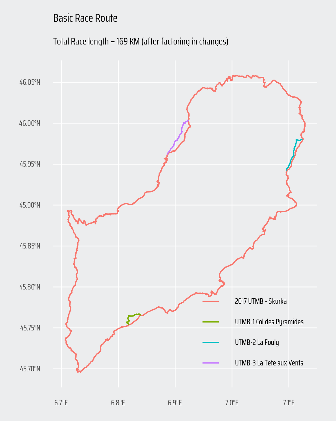
Basic Plot fo the Race Route
This code calculates the total length of the UTMB ultramarathon route in kilometers using the spatial data manipulation capabilities of the {sf} package. It then visualizes the route with a basic map, highlighting the total race length in the subtitle. The map is styled using {ggplot2} from {tidyverse}, and the final plot is saved to a file using {ggsave}. Custom themes and labels enhance the presentation, making it suitable for publication-quality outputs.
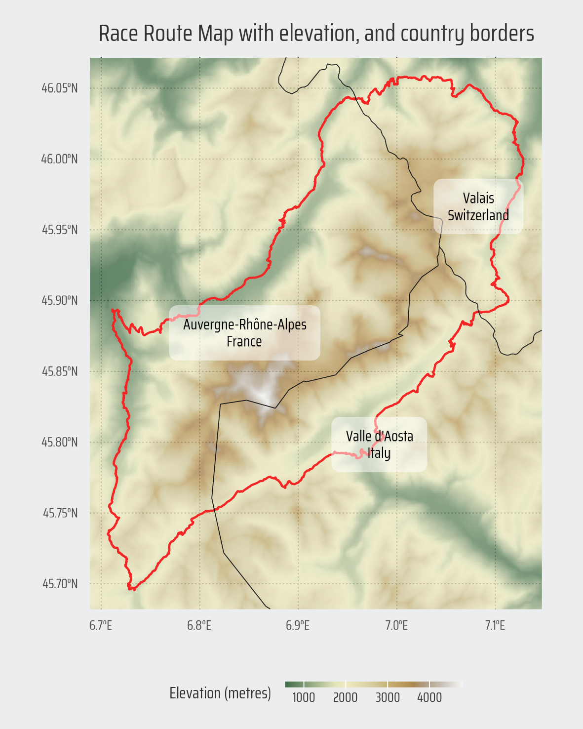
Add background map of elevation, country’s borders and names.
This code chunk processes spatial data to create an elevation map of the UTMB race route with country borders. Using the sf package, it creates a buffered boundary around the route for cropping elevation rasters fetched via elevatr. National borders are retrieved using geodata and refined through spatial operations (st_crop, st_difference) to isolate inner boundaries. The visualization combines terra raster data, tidyterra for ggplot integration, and custom styling to highlight the route against a shaded relief backdrop.
Code
# Bounding Boxes and Cropping areas for display of Race Route# An sf object to use for cropping rasters and vectorsmap_boundary_crop_vector <- utmb_route |>slice(1) |>st_geometry() |># Add a buffer of 1 km around race track for rasterst_buffer(dist =1000)# A bounding box to get elevation and maps datautmb_bbox <- map_boundary_crop_vector |>st_bbox()# Elevation Raster for the Race Area -----------------------------raw_raster <- elevatr::get_elev_raster( utmb_route,z =10)elevation_raster <- raw_raster |>rast() |> terra::crop( map_boundary_crop_vector, extend =TRUE, )# Getting Countries Maps and borders ----------------------------# raw_borders <- geodata::gadm(# country = c("FRA", "ITA", "CHE"),# level = 2,# path = tempdir(),# resolution = 1# )raw_borders_national <- geodata::gadm(country =c("FRA", "ITA", "CHE"),level =1,path =tempdir(),resolution =1)# borders_vec <- raw_borders |> # st_as_sf() |> # st_transform("EPSG:4326") |> # janitor::clean_names() |> # st_crop(utmb_bbox) |> # select(country, name_1, name_2, geometry)borders_vec_labels <- raw_borders_national |>st_as_sf() |>st_transform("EPSG:4326") |> janitor::clean_names() |>st_crop(utmb_bbox) |>select(country, name_1, geometry)# Make another sf object to keep only inner borders -----------------# and remove the outer box (for nicer plotting) ---------------------# Prepare sf object of polygons and Ensure it's validall_borders <-st_make_valid(borders_vec_labels) |># Get all polygon borders as multilinestringsst_cast("MULTILINESTRING") |>st_transform("EPSG:3857") |>st_union()# Dissolve all polygons into one to get outer boundaryouter_borders <-st_union(borders_vec_labels) |>st_cast("MULTILINESTRING") |>st_transform("EPSG:3857") |>st_buffer(1)# Remove outer boundary from all borders → keep innerinner_borders <-st_difference( all_borders, outer_borders ) |>st_transform("EPSG:4326")rm(all_borders, outer_borders)# ------------------------------------------------------------------g <-ggplot() +geom_spatraster(data = elevation_raster,maxcell =Inf,alpha =0.8 ) +scale_fill_wiki_c() +geom_sf(data = utmb_route |>slice(1) |>st_geometry(),colour = mypal[1] ) +geom_sf(data = inner_borders,fill =NA,linewidth =0.2,colour ="grey10" ) +geom_sf_label(data = borders_vec_labels,mapping =aes(label =paste0(name_1, "\n", country)),lineheight =0.3,family ="body_font",fill =alpha(mypal[6], 0.5),label.size =NA,size =8 ) +coord_sf(expand =FALSE) +labs(x =NULL,y =NULL,title ="Race Route Map with elevation, and country borders",fill ="Elevation (metres) " ) +theme_minimal(base_size =24,base_family ="body_font" ) +theme(legend.position ="bottom",text =element_text(margin =margin(0,0,0,0, "mm"),colour ="grey20",hjust =0.5 ),plot.title =element_text(margin =margin(0,0,2,0, "mm"),hjust =0.5,size =36 ),axis.text.x =element_text(margin =margin(2,0,0,0, "mm") ),axis.text.y =element_text(margin =margin(0,2,0,0, "mm") ),legend.box.margin =margin(0,0,0,0, "mm"),legend.margin =margin(0,0,0,0, "mm"),axis.ticks.x =element_blank(),axis.ticks.length.x =unit(0, "mm"),axis.ticks.y =element_blank(),axis.ticks.length.y =unit(0, "mm"),legend.text =element_text(margin =margin(1,0,0,0, "mm") ),legend.title =element_text(margin =margin(0,2,0,0, "mm") ),legend.key.height =unit(1, "mm"),panel.grid =element_line(linewidth =0.2,colour ="black",linetype =3 ) )ggsave(plot = g,filename = here::here("geocomputation", "images","utmb_ultramarathon_2.png" ),units ="cm",height =10*5/4, width =10,bg = bg_col)
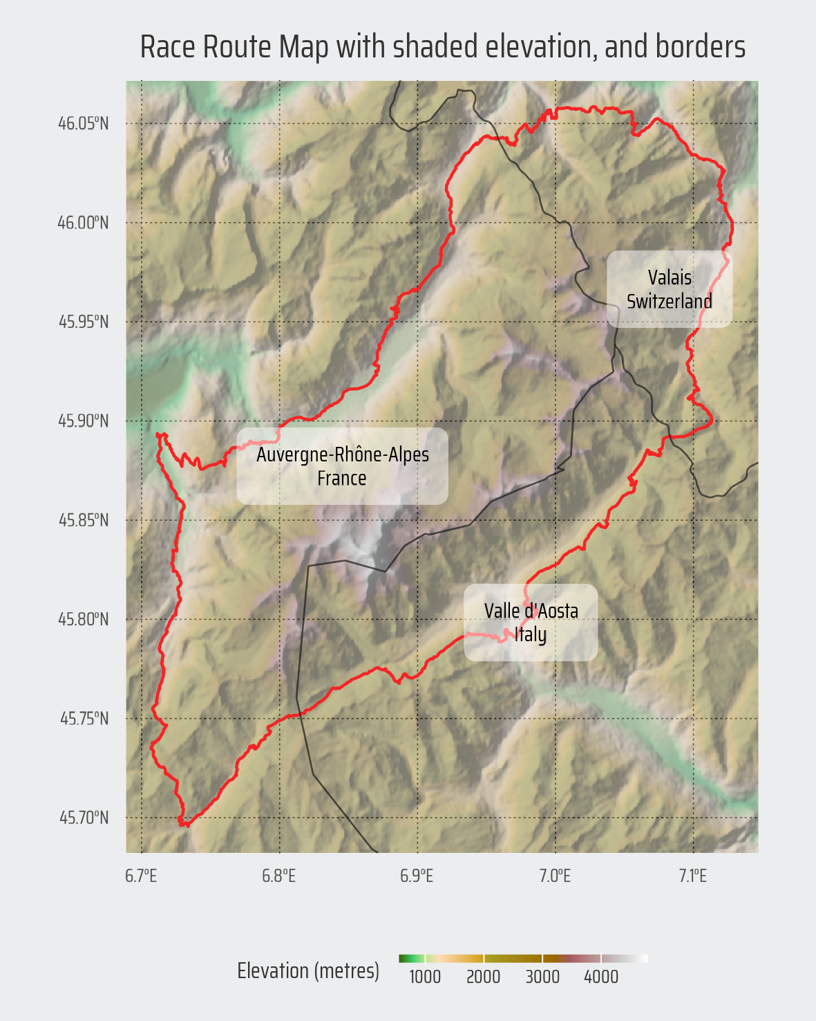
This code enhances the UTMB race map by creating a shaded relief visualization using terra for raster processing and whitebox’s multidirectional hillshade algorithm to simulate realistic terrain shadows. The geom_spatraster from tidyterra layers both elevation data and hillshade, while ggblend merges them with a “multiply” blend mode for depth. paletteer provides the grayscale hillshade palette, and scale_fill_hypso_c adds elevation coloring. The final map overlays the route (via sf) and borders for a professional topographic presentation.
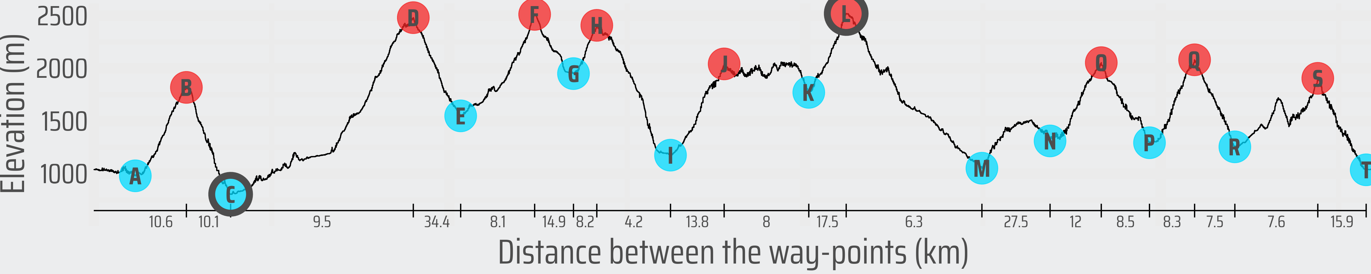
This code extracts elevation values for evenly spaced points along the UTMB race route to create a detailed elevation profile. Using sf, the route is segmented into 100-meter intervals and converted to points, while elevation data is retrieved using terra and extract. Key waypoints, including the highest and lowest elevation points, are identified and labeled. The visualization combines elevation trends with annotated waypoints for a clear depiction of the route’s altitude dynamics.
Code
path_points <- utmb_route |># Keep only the main routeslice(1) |>select(name, geometry) |># Convert to non-geographic CRS to save huge computational timest_transform("EPSG:3857") |># Convert multi-linestring to line-stringst_cast("LINESTRING") |># Break into line segments of 100 metres eachst_segmentize(dfMaxLength =100) |># Convert each line segment into a central point# to be able to extract its elevationst_cast("POINT")# Obtain Coordinates of each pointpoint_coordinates <-st_coordinates(path_points)# compute distance of each point from the start point_distances <-c(0, cumsum(sqrt(rowSums(diff(point_coordinates)^2 ) ) ) )# Add distance from starting point as a column, and# re-convert back to Geographic CRSpath_points <- path_points |>mutate(dist = point_distances) |>st_transform("EPSG:4326")# Get corresponding elevation values for each point along race routeelevation_raw_values <- terra::extract( elevation_raster, path_points ) |>as_tibble() |>select(2) |>pull()# Final elevation dataroute_elevation <- path_points |>mutate(elev_value = elevation_raw_values,dist =as.numeric(dist),id =row_number() ) |>select(-name) |>relocate(id)rm(elevation_raw_values, path_points)# Check "dist" variable# ggplot(route_elevation) +# geom_point(# aes(x = id, y = dist)# )# It Works!!# Check the Elevation Variable# ggplot(route_elevation) +# geom_point(aes(x = id, y = elev_value))# It Works!!# Get Additional Information -------------------------------------# Lowest and highest points along the routeroute_extremes <- route_elevation |>slice_min(elev_value, n =1, with_ties =FALSE) |>bind_rows( route_elevation |>slice_max(elev_value, n =1, with_ties =FALSE) ) |>st_drop_geometry() |>mutate(extreme_points =TRUE )# Manually select the route trend points# A basic ggplot2 to get top most pointsroute_elevation |>arrange(desc(elev_value)) |>ggplot(aes(id, elev_value)) +geom_line() +geom_text(aes(label = id),check_overlap = T )selected_points_high <-c(651, 2246, 3099, 3536, 4431, 5289, 7082, 7738, 8604)# A basic ggplot2 to get lowest pointsroute_elevation |>arrange(elev_value) |>ggplot(aes(id, elev_value)) +geom_line() +geom_text(aes(label = id),check_overlap = T )selected_points_low <-c(292, 962, 2579, 3372, 4054, 5026, 6243, 6722, 7421, 8021, 8944)route_elevation_df <- route_elevation |>mutate(waypoint_type =case_when( id %in% selected_points_high ~"High Point", id %in% selected_points_low ~"Low Point",.default =NA ) ) |>left_join(route_extremes)# Get an X-Axis data: distance between selected waypointswaypoints_df <- route_elevation_df |>filter(!is.na(waypoint_type)) |>mutate(xmin_var = id,xmax_var =lead(id),xmean_var = (xmax_var + xmin_var)/2,xlab_var =round((dist -lag(dist))/1e3, 1) )waypoints_df$xmin_var[1] <-0waypoints_df$xlab_var[1] <-round((waypoints_df$dist[1])/1000, 1) waypoints_df$waypoint_label <- LETTERS[1:nrow(waypoints_df)]# Start the plotg_inset <-ggplot() +geom_line(data = route_elevation,mapping =aes(x = id,y = elev_value ) ) +geom_segment(data = waypoints_df,mapping =aes(y =650,yend =650,x = xmin_var,xend = xmax_var ),arrow =arrow(angle =90, length =unit(2, "mm")) ) +# Add high-points and low-pointsgeom_point(data = waypoints_df,mapping =aes(x = id, y = elev_value,colour = waypoint_type ),size =12,alpha =0.75 ) +scale_colour_manual(values = mypal[c(1,2)] ) +geom_text(data = waypoints_df,mapping =aes(x = id, y = elev_value,label = waypoint_label ),size = bts /4,family ="body_font",colour = text_col,fontface ="bold" ) +# X-Axis Textgeom_text(data = waypoints_df,mapping =aes(x = xmean_var,y =600,label = xlab_var ),vjust =1,hjust =0.5,colour = text_col,size = bts /6,family ="body_font" ) +# Add extremes - highest and lowestgeom_point(data = waypoints_df |>filter(extreme_points),mapping =aes(x = id, y = elev_value),pch =21,fill =NA, colour = text_col,stroke =4,size =12 ) +scale_x_continuous(expand =expansion(0) ) +labs(y ="Elevation (m)",x ="Distance between the way-points (km)" ) +coord_cartesian(clip ="off") +theme_minimal(base_family ="body_font",base_size = bts ) +theme(plot.margin =margin(1,0,1,0, "mm"),text =element_text(colour = text_col ),axis.text.x =element_blank(),axis.ticks.x =element_blank(),axis.ticks.length.x =unit(0, "mm"),axis.title.x =element_text(margin =margin(4,0,0,0, "mm") ),axis.text.y =element_text(margin =margin(0,2,0,0, "mm"),colour = text_col ),axis.title.y =element_text(margin =margin(0,1,0,0, "mm") ),axis.ticks.length.y =unit(0, "mm"),legend.position ="none" )ggsave(plot = g_inset,filename = here::here("geocomputation", "images","utmb_ultramarathon_4.png" ),height =8,width =40,units ="cm",bg = bg_col)
Figure 5
Composing Final Plot
This code creates a comprehensive visual representation of the UTMB ultramarathon route, combining a shaded relief elevation map with the race path and country borders. It utilizes ggplot2 for plotting, sf for spatial data manipulation, and terra for raster processing. The map includes annotations for key points such as the start, highest, and lowest elevations, along with manually selected waypoints. An inset elevation profile, created using ggblend for layer blending, provides additional context. The final plot is customized with detailed themes and annotations to enhance readability and visual appeal.
Figure 6: The Final Composed Plot with {patchwork}
Remove temporary files
Code
# Remove the temporary files:# "Do no harm and leave the world an untouched place"unlink(here::here("geocomputation", "images","temp_utmb_ultramarathon_2.tiff"))unlink(here::here("geocomputation", "images","temp_utmb_ultramarathon.tiff"))
Interactive Map
This interactive visualization leverages the leaflet package via mapview to create an explorable UTMB route map. Dynamic popups at waypoints display elevation, distances etc. using sf-processed spatial data. The base map utilizes OpenStreetMap or OpenTopoMap layers. Elevation trends are derived from elevatr-generated DEM data.
Code
### THE ACTUAL CODE USED TO PRODUCE A CONSICE OUTPUT SF OBJECT### TO SAVE RENDERING TIME, THE OUTPUT OBJECT IS SAVED# # An sf object to use for cropping rasters and vectors# map_boundary_crop_vector <- utmb_route |> # slice(1) |> # st_geometry() |> # # Add a buffer of 1 km around race track for raster# st_buffer(dist = 1000)# # raw_raster <- elevatr::get_elev_raster(# utmb_route,# z = 10# )# # elevation_raster <- raw_raster |> # rast() |> # terra::crop(# map_boundary_crop_vector, # extend = TRUE,# )# # path_points <- utmb_route |> # # # Keep only the main route# slice(1) |> # select(name, geometry) |> # # # Convert to non-geographic CRS to save huge computational time# st_transform("EPSG:3857") |> # # # Convert multi-linestring to line-string# st_cast("LINESTRING") |> # # # Break into line segments of 100 metres each# st_segmentize(dfMaxLength = 100) |> # # # Convert each line segment into a central point# # to be able to extract its elevation# st_cast("POINT")# # # Obtain Coordinates of each point# point_coordinates <- st_coordinates(path_points)# # # compute distance of each point from the start # point_distances <- c(# 0, # cumsum(# sqrt(# rowSums(# diff(point_coordinates)^2# )# )# )# # )# # # # Extract only the first column (i.e. the distance from# # first point alone). Otherwise, st_distance() # # returns a distance matrix As expected, distance grows # # by approx. less than dfMaxLength amount per points# path_points <- path_points |> # mutate(dist = point_distances) |> # st_transform("EPSG:4326")# # # Get corresponding elevation values for each point along race route# elevation_raw_values <- terra::extract(# elevation_raster, path_points# ) |> # as_tibble() |> # select(2) |> # pull()# # # Final elevation data# route_elevation <- path_points |> # mutate(# elev_value = elevation_raw_values,# dist = as.numeric(dist),# id = row_number()# ) |> # select(-name) |> # relocate(id)# # rm(elevation_raw_values,# path_points)# # # # Check "dist" variable# ggplot(route_elevation) +# geom_point(# aes(x = id, y = dist)# )# # It Works!!# # # Check the Elevation Variable# ggplot(route_elevation) +# geom_point(aes(x = id, y = elev_value))# # It Works!!# # # Get Additional Information -------------------------------------# # Lowest and highest points along the route# route_extremes <- route_elevation |> # slice_min(elev_value, n = 1, with_ties = FALSE) |> # bind_rows(# route_elevation |> # slice_max(elev_value, n = 1, with_ties = FALSE)# ) |># st_drop_geometry() |> # mutate(# extreme_points = TRUE# )# # # # Manually select the route trend points# # A basic ggplot2 to get top most points# route_elevation |># arrange(desc(elev_value)) |># ggplot(aes(id, elev_value)) +# geom_line() +# geom_text(# aes(label = id),# check_overlap = T# )# # selected_points_high <- c(651, 2246, 3099, 3536, 4431, # 5289, 7082, 7738, 8604)# # A basic ggplot2 to get lowest points# route_elevation |># arrange(elev_value) |># ggplot(aes(id, elev_value)) +# geom_line() +# geom_text(# aes(label = id),# check_overlap = T# )# # selected_points_low <- c(292, 962, 2579, 3372, 4054, 5026, # 6243, 6722, 7421, 8021, 8944)# # route_elevation_df <- route_elevation |> # mutate(# waypoint_type = case_when(# id %in% selected_points_high ~ "High Point",# id %in% selected_points_low ~ "Low Point",# .default = NA# )# ) |> # left_join(route_extremes)# # # Save the complete analysis resutl (to save computation time)# saveRDS(# route_elevation_df,# file = here::here("data", "utmb_route_elevation.rds")# )route_elevation_df <-readRDS(here::here("data", "utmb_route_elevation.rds"))# Get data: distance between selected waypointswaypoints_df <- route_elevation_df |>filter(!is.na(waypoint_type) | id ==1) |>mutate(xmin_var = id,xmax_var =lead(id),xmean_var = (xmax_var + xmin_var)/2,xlab_var =round((dist -lag(dist))/1e3, 1) ) |>mutate(waypoint_type =if_else(is.na(waypoint_type), "Starting Point", waypoint_type),xlab_var =if_else(id ==1, 0, xlab_var),waypoint_label = LETTERS[1:nrow( route_elevation_df |>filter(!is.na(waypoint_type) | id ==1) )] ) |>mutate(`Waypoint Name`= waypoint_label,`Distance from Starting Point`=paste0(round(dist /1e3, 1)," km"),`Elevation`=paste0(elev_value, " metres"),`Distance from last waypoint`=paste0(round(xlab_var, 1)," km") )`UTMB Race Route`<- utmb_route |>slice(1) |>select(geometry)mapview(`UTMB Race Route`, color ="red", alpha =0.9,legend =FALSE,map.types =c("OpenStreetMap.Mapnik","OpenTopoMap"),lwd =4,popup =FALSE ) +mapview( waypoints_df,zcol ="waypoint_type",col.regions =c("darkred", "blue", "green"),alpha =0.9,popup =popupTable( waypoints_df,zcol =c("Waypoint Name", "Distance from Starting Point", "Elevation", "Distance from last waypoint"),feature.id =FALSE,row.numbers =FALSE ),layer.name ="Waypoints",legend =TRUE,legend.pos ="bottomright",legend.opacity =0.5 )
Figure 7: Interactive Version of the Ultra-Trail du Mont-Blanc (UTMB) Route, with selected way-points