Chapter 17

Factors

Author

Aditya Dahiya

Published

September 14, 2023

library(tidyverse)
library(ggthemes)
library(gt)
library(gtExtras)
data("gss_cat")

Important Points

Most rename and recoding functions in the tidyverse, the new values go on the left and the old values go on the right.

17.3.1 Exercise

Question 1

Explore the distribution of rincome (reported income). What makes the default bar chart hard to understand? How could you improve the plot?

The default bar chart is hard to understand because: –

It is vertical, and the names of categories overlap on x-axis.
The “Not applicable” category is before the lowest income group. Thus, the pattern is disturbed.

We could improve the plot, as shown in Figure 1, by: —

Making it into a horizontal bar chart to allow space and easy reading of categories of income levels.
Move the “Not Applicable” level after the highest income level, along-side “Refused”, “Dont’ know” and “No answer”.
Further, we could remove non-data ink, as per principles of Mr. Tufte to make our pattern stand out. Also, we could create a separate colouring scheme for data outside the income levels.

no_levels = levels(gss_cat$rincome)[c(1:3, 16)]

gss_cat |>
  mutate(col_level = rincome %in% no_levels) |>
  ggplot(aes(y = fct_relevel(rincome, 
                             "Not applicable",
                             after = 3),
             fill = col_level)) +
  geom_bar() +
  theme_minimal() +
  labs(x = "Number of respondents", y = NULL,
       title = "Income Levels of respondents in General Social Survey") +
  theme(panel.grid.major = element_blank(),
        panel.grid.minor = element_blank(),
        legend.position = "none") +
  scale_fill_manual(values = c("#3d3b3b", "#999494"))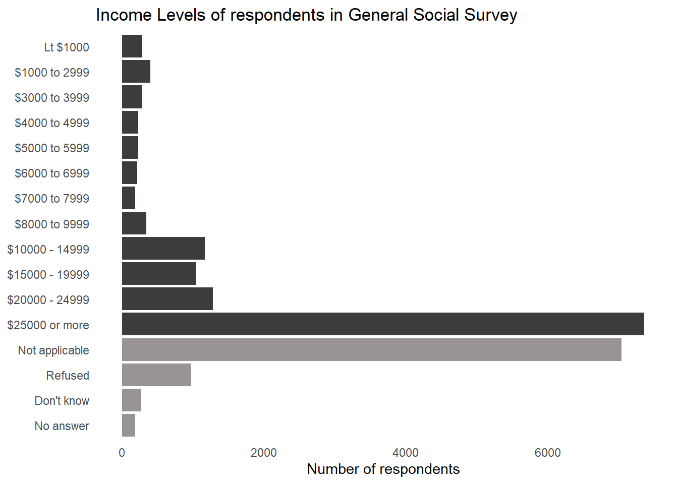

Question 2

What is the most common relig in this survey? What’s the most common partyid?

The most common relig is “Protestant”. And, the most common partyid is “Independent”.

gss_cat |>
  count(relig, sort = TRUE)

# A tibble: 15 × 2
   relig                       n
   <fct>                   <int>
 1 Protestant              10846
 2 Catholic                 5124
 3 None                     3523
 4 Christian                 689
 5 Jewish                    388
 6 Other                     224
 7 Buddhism                  147
 8 Inter-nondenominational   109
 9 Moslem/islam              104
10 Orthodox-christian         95
11 No answer                  93
12 Hinduism                   71
13 Other eastern              32
14 Native american            23
15 Don't know                 15

gss_cat |>
  count(partyid, sort = TRUE)

# A tibble: 10 × 2
   partyid                n
   <fct>              <int>
 1 Independent         4119
 2 Not str democrat    3690
 3 Strong democrat     3490
 4 Not str republican  3032
 5 Ind,near dem        2499
 6 Strong republican   2314
 7 Ind,near rep        1791
 8 Other party          393
 9 No answer            154
10 Don't know             1

Question 3

Which relig does denom (denomination) apply to? How can you find out with a table? How can you find out with a visualization?

We can see from the code below that more than one factor values in denom (denomination) occur only in “Protestant”, “Christian” and “Other” religions. To explore further, we can cross-tabulate religion and denomination, as shown in Table 1, and realize that the only religion to which denomination really applies to is “Protestant”.

We could also do a visualization as in Figure 2 .

gss_cat |>
  group_by(relig) |>
  summarise(n = n_distinct(denom)) |>
  arrange(desc(n)) |>
  filter(n > 1)

# A tibble: 3 × 2
  relig          n
  <fct>      <int>
1 Protestant    29
2 Christian      4
3 Other          2

gss_cat |>
  filter(relig %in% c("Protestant", "Christian", "Other")) |>
  group_by(relig, denom) |>
  tally() |>
  spread(relig, n) |>
  arrange(desc(Christian)) |>
  gt() |>
  sub_missing(missing_text = "") |>
  gt_theme_538()

Table 1:
Cross-Table of the deominations within the three religions
denom	Christian	Other	Protestant
No denomination	452	7	1224
Not applicable	224	217
Don't know	11		41
No answer	2		22
Other			2534
Episcopal			397
Presbyterian-dk wh			244
Presbyterian, merged			67
Other presbyterian			47
United pres ch in us			110
Presbyterian c in us			104
Lutheran-dk which			267
Evangelical luth			122
Other lutheran			30
Wi evan luth synod			71
Lutheran-mo synod			212
Luth ch in america			71
Am lutheran			146
Methodist-dk which			239
Other methodist			33
United methodist			1067
Afr meth ep zion			32
Afr meth episcopal			77
Baptist-dk which			1457
Other baptists			213
Southern baptist			1536
Nat bapt conv usa			40
Nat bapt conv of am			76
Am bapt ch in usa			130
Am baptist asso			237

gss_cat |>
  group_by(relig) |>
  summarise(n = n_distinct(denom)) |>
  arrange(desc(n)) |>
  ggplot(aes(y = reorder(relig, n), x = n)) +
  geom_bar(stat = "identity") +
  theme_minimal() +
  labs(x = "Number of denominations", y = NULL,
       title = "Only Protestant religion has demoninations within it")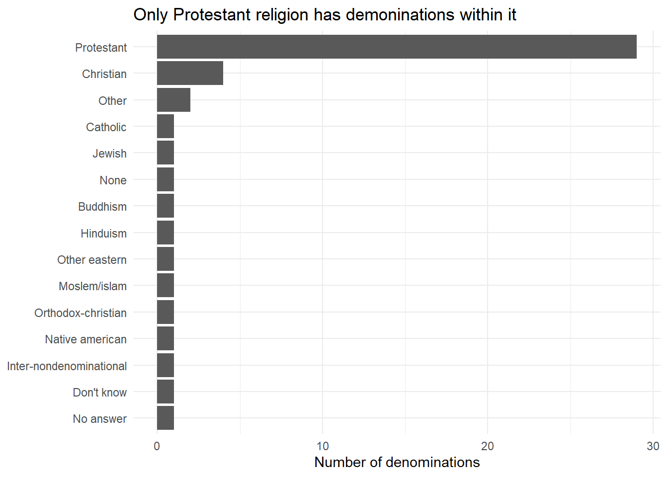

17.4.1 Exercises

Question 1

There are some suspiciously high numbers in tvhours. Is the mean a good summary?

No, mean is not a good summary as the distribution of tvhours is right skewed. Instead, we should use median as a summary measure.

gss_cat |>
  drop_na() |>
  mutate(tvhours = as_factor(tvhours)) |>
  ggplot(aes(x = tvhours)) +
  geom_bar(col = "black", fill = "white") +
  theme_clean() +
  labs(x = "Hours per day spent watching TV",
       y = "Numbers", title = "Distribution of TV Hours is right skewed")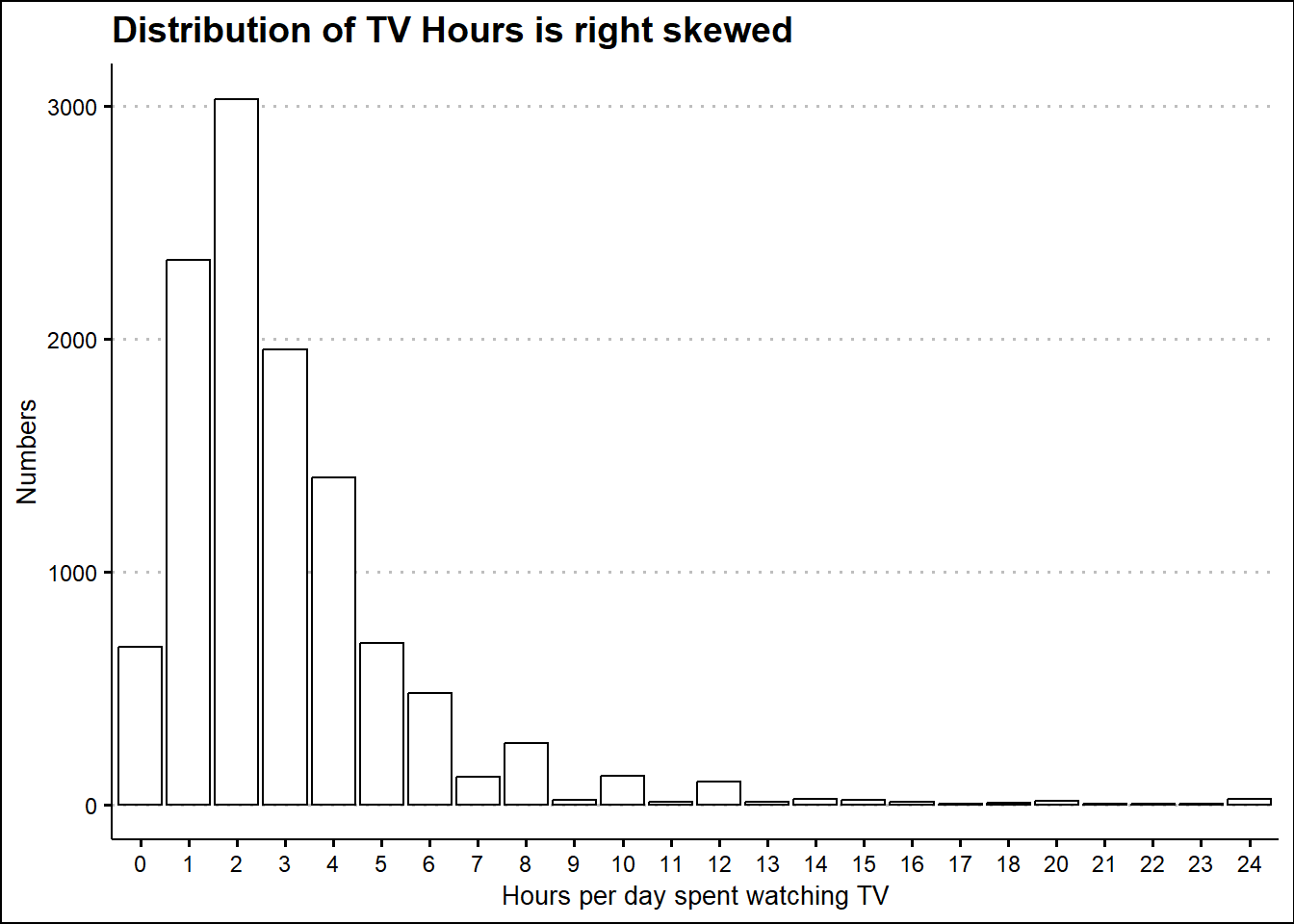

Question 2

For each factor in gss_cat identify whether the order of the levels is arbitrary or principled.

The variables in the gss_cat data-set which are factors are: —

Factor Variable	Levels	Order is arbitrary or principled
`marital`	No answer, Never married, Separated, Divorced, Widowed and, Married	Arbitrary, since they are not in a specific order
`race`	Other, Black, White and, Not applicable	Arbitrary, since they are not in a specific order
`rincome`	No answer, Don’t know, Refused, $25000 or more, $20000 - 24999, $15000 - 19999, $10000 - 14999, $8000 to 9999, $7000 to 7999, $6000 to 6999, $5000 to 5999, $4000 to 4999, $3000 to 3999, $1000 to 2999, Lt $1000 and, Not applicable	Principled, since the income levels are in a specified increasing or decreasing order, with few levels arbitrary
`partyid`	No answer, Don’t know, Other party, Strong republican, Not str republican, Ind,near rep, Independent, Ind,near dem, Not str democrat and, Strong democrat	Partly Principled, as there are two extremes, and then levels in the middle.
`relig`	No answer, Don’t know, Inter-nondenominational, Native american, Christian, Orthodox-christian, Moslem/islam, Other eastern, Hinduism, Buddhism, Other, None, Jewish, Catholic, Protestant and, Not applicable	Arbitrary, as the religions are not in a specific order.
`denom`	No answer, Don’t know, No denomination, Other, Episcopal, Presbyterian-dk wh, Presbyterian, merged, Other presbyterian, United pres ch in us, Presbyterian c in us, Lutheran-dk which, Evangelical luth, Other lutheran, Wi evan luth synod, Lutheran-mo synod, Luth ch in america, Am lutheran, Methodist-dk which, Other methodist, United methodist, Afr meth ep zion, Afr meth episcopal, Baptist-dk which, Other baptists, Southern baptist, Nat bapt conv usa, Nat bapt conv of am, Am bapt ch in usa, Am baptist asso and, Not applicable	Arbitrary, as the denominations are not in a specific order.

Question 3

Why did moving “Not applicable” to the front of the levels move it to the bottom of the plot?

Moving “Not applicable” to the front of the levels move it to the bottom of the plot, because ggplot2 plots the levels in increasing order, starting bottom’s upwards.

17.5.1 Exercises

Question 1

How have the proportions of people identifying as Democrat, Republican, and Independent changed over time?

As reflected in the Figure 3, the proportions of people identifying as Democrat has slightly increased, Republican has slightly decreased, and Independent has increased, over the period of 15 years reflected in the data-set.

gss_cat |>
  mutate(
    partyid = fct_collapse(partyid,
      "Republican"  = c("Strong republican",  "Not str republican"),
      "Democrat"    = c("Strong democrat", "Not str democrat"),
      "Independent" = c("Independent", "Ind,near dem", "Ind,near rep"),
      "Others"      = c("No answer", "Don't know", "Other party")
    )
  ) |>
  group_by(year, partyid) |>
  count() |>
  ggplot(aes(x = year, y = n, fill = partyid)) +
  geom_col(position = "fill") +
  scale_fill_manual(values = c("lightgrey", "red", "grey", "blue")) +
  theme_classic() +
  theme(legend.position = "bottom") +
  labs(x = "Year", y = "Proportion of respondents", fill = "Party",
       subtitle = "Proportion of republicans has decreased, while that of independents has increased over the years",
       title = "In 15 years, share of parties' supporters has changed")

Figure 3: Stacked bar chart of the partyid in the data-set

Question 2

How could you collapse rincome into a small set of categories?

We could collapse the rincome into a small set of categories using the following functions: –

fct_lump_n()
fct_lump_lowfreq()
fct_lump_min()
fct_lump_prop()
fct_lump()
fct_collapse()

gss_cat|>
  mutate(
    rincome = fct_lump_n(rincome, n = 6)
  ) |>
  group_by(rincome) |>
  count() |>
  arrange(desc(n)) |>
  ungroup() |>
  gt() |>
  cols_label(rincome = "Annual Income",
             n = "Numbers")

Annual Income	Numbers
$25000 or more	7363
Not applicable	7043
Other	2603
$20000 - 24999	1283
$10000 - 14999	1168
$15000 - 19999	1048
Refused	975

Question 3

Notice there are 9 groups (excluding other) in the fct_lump example above. Why not 10? (Hint: type ?fct_lump, and find the default for the argument other_level is “Other”.)

Yes, there are 9 groups (excluding other) in this example, as shown below also in Figure 4. This is because n = 10 argument limits the total groups to 10, and the function needs one group for “Other”, i.e. all other groups whose count is lesser than top 9 groups. Thus, the groups shown are 9, with 1 as “Other” (at the end).

gss_cat |>
  mutate(relig = fct_lump_n(relig, n = 10)) |>
  count(relig) |>
  gt()

relig	n
Inter-nondenominational	109
Christian	689
Orthodox-christian	95
Moslem/islam	104
Buddhism	147
None	3523
Jewish	388
Catholic	5124
Protestant	10846
Other	458

Figure 4: Table of number of respondents from each of top 10 religions, including Other