# Load libraries
library(tidyverse)
library(rvest)
library(gt)
library(gtExtras)
library(scales)Chapter 25
Web scraping
In the realm of aviation history and military technology, fighter aircraft hold a pivotal role, representing the pinnacle of technological prowess and strategic significance. To delve into the comprehensive landscape of fighter aircraft, this assignment embarks on a journey of data acquisition and analysis, leveraging the versatile capabilities of the R programming language, specifically the rvest package(Wickham 2022) within the tidyverse framework(Wickham et al. 2019).
Our primary data source, the Wikipedia page titled “List of Fighter Aircraft,” serves as a repository of valuable information encompassing various facets of fighter aircraft production, categorization, and operational status.
This page aims to meticulously extract, process, and analyze the data from this source, shedding light on the countries that have contributed significantly to fighter aircraft production, the prevailing types of aircraft that have dominated the skies, and the intriguing disparities between operational and retired aircraft, including the number of prototypes produced. Through this endeavor, we endeavor to gain profound insights into the historical and contemporary dynamics of fighter aircraft, uncovering patterns and trends that illuminate their pivotal role in military aviation and defense strategies.
Experiment scraping the Wikipedia page of fighter aircraft
# The web-address to harvest
url <- "https://en.wikipedia.org/wiki/List_of_fighter_aircraft"

# Read in the html file from the URL
url_html <- read_html(url)

# Create a nice looking tibble from the data
df <- url_html |>
  html_element("table") |>
  html_table() |>

  # house-keeping tasks: cleaning names etc.
  janitor::clean_names() |>
  rename(
    numbers = no,
    year = date
  ) |>
  select(-notes) |>
  mutate(
    numbers = parse_number(numbers),
    class = str_replace_all(class,
                            pattern = "\"",
                            replacement = ""),
    class = na_if(class, ""),
    status = fct(status, levels = c("Abandoned",
                                    "Prototype",
                                    "In Development",
                                    "Retired",
                                    "Operational"))
  )
Displaying the complete data, in a nicely formatted table at Figure 1 : –
df |>
  gt() |>
  cols_label_with(fn = ~ janitor::make_clean_names(., "title")) |>
  opt_interactive(page_size_default = 5,
                  use_highlight = TRUE,
use_resizers = TRUE)Using the data for some analysis
In order to visually convey the the total number of fighter aircraft manufactured by each nation, we employ the powerful visualization tool provided by Datawrapper, and create a pie chart: –
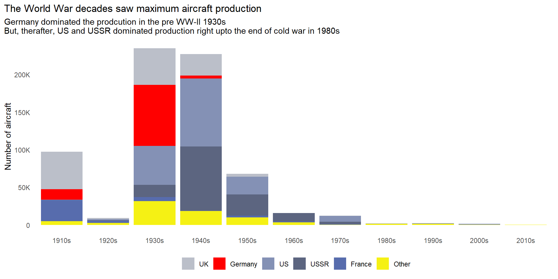
Now, we will visualize the production of fighter aircraft over different decades, categorized by their design years and attributed to various countries, using a stacked bar chart in Figure 2 .
# A stacked bar chart for country-wise aircraft made in each decade

df |>
  mutate(
    country = fct(country),
    decade = fct(paste0(floor(year / 10) * 10, "s"),
                 levels = paste0(seq(1910, 2020, by = 10), "s"))
  ) |>
  group_by(decade, country) |>
  count(wt = numbers,
        name = "nos_planes") |>

  # Ungroup so that factor lumping works
  ungroup() |>

  # Remove 2020s as very few observations; and irrelevant to the message
  filter(decade != "2020s") |>

  # Lump into 5 factors for easy display of coloured stacked bar chart
  mutate(country = fct_lump_n(country, n = 5, w = nos_planes)) |>

  # Start plotting
  ggplot(aes(x = decade,
             y = nos_planes,
             fill = country,
             label = country,
             text = paste0("Aircrafts produced in the decade: ", nos_planes))
         ) +
  geom_bar(stat = "identity",
           position = "stack") +
  scale_y_continuous(labels = label_number_si()) +
  labs(x = NULL,
       y = "Number of aircraft",
       title = "The World War decades saw maximum aircraft production",
       subtitle = "Germany dominated the prodcution in the pre WW-II 1930s\nBut, therafter, US and USSR dominated production right upto the end of cold war in 1980s",
       fill = NULL) +
  scale_fill_manual(values = c("#bbbfc9",
                               "red",
                               "#8491b5",
                               "#5c6580",
                               "#576cad",
                               "#f5f114")) +
  guides(fill = guide_legend(nrow = 1)) +
  theme_minimal() +
  theme(legend.position = "bottom",
        panel.grid = element_blank(),
        plot.title.position = "plot")
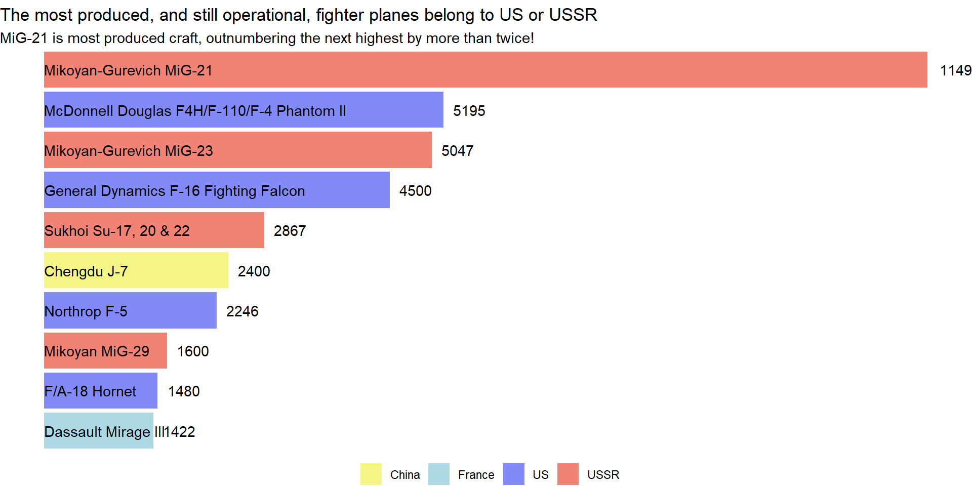
Here in Figure 3 are the most produced operational aircraft still operational as of today.
df |>
  filter(status == "Operational") |>
  arrange(desc(numbers)) |>
  slice_head(n = 10) |>
  mutate(type = if_else(type == "McDonnell Douglas F/A-18 Hornet",
                        "F/A-18 Hornet",
                        type)) |>
  ggplot(aes(x = numbers,
             y = reorder(type, numbers),
             fill = country)) +
  geom_bar(stat = "identity") +
  theme_void() +
  geom_text(aes(x = 0,
                label = type),
            hjust = "left") +
  geom_text(aes(label = numbers),
            hjust = -0.3) +
  labs(fill = NULL,
       title = "The most produced, and still operational, fighter planes belong to US or USSR",
       subtitle = "MiG-21 is most produced craft, outnumbering the next highest by more than twice!")  +
  scale_fill_manual(values = c("#f5f584", "lightblue", "#828afa", "#f28374")) +
  theme(plot.title.position = "panel",
        legend.position = "bottom")
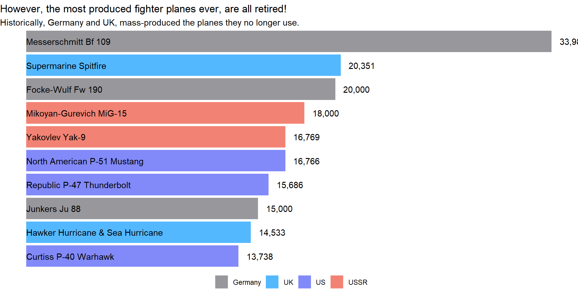
But, if we look at the most mass-produced ever made, all of them are retired as shown below in Figure 4 .
df |>
  arrange(desc(numbers)) |>
  slice_head(n = 10) |>
  ggplot(aes(x = numbers,
             y = reorder(type, numbers),
             fill = country)) +
  geom_bar(stat = "identity") +
  theme_void() +
  geom_text(aes(x = 0,
                label = type),
            hjust = "left") +
  geom_text(aes(label = scales::comma(numbers)),
            hjust = -0.3) +
  labs(fill = NULL,
       title = "However, the most produced fighter planes ever, are all retired!",
       subtitle = "Historically, Germany and UK, mass-produced the planes they no longer use.")  +
  scale_fill_manual(values = c("#97979c", "#54b8ff", "#828afa", "#f28374")) +
  theme(plot.title.position = "panel",
        legend.position = "bottom")
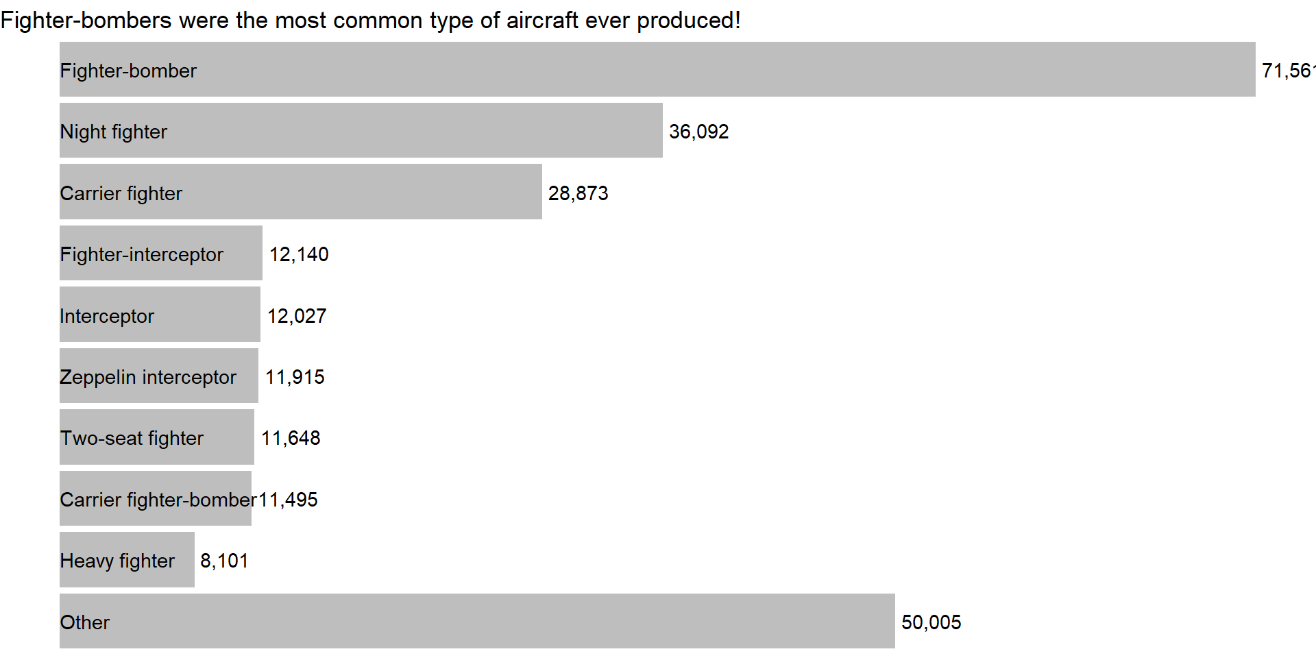
Now, looking at the class of aircraft, the most produced type of aircraft, all time are shown in Figure 5 .
df |>
  mutate(class = if_else(class == "fighter-bomber",
                         "Fighter-bomber",
                         class)) |>
  count(class, sort = TRUE, wt = numbers) |>
  drop_na() |>
  mutate(
    class = fct(class),
    class = fct_lump_n(class, n = 9, w = n)
  ) |>
  count(class, sort = TRUE, wt = n) |>
  ggplot(aes(x = n,
             y = fct_rev(class))) +
  geom_bar(stat = "identity", fill = "grey") +
  theme_void() +
  geom_text(aes(x = 0,
                label = class),
            hjust = "left") +
  geom_text(aes(label = scales::comma(n)),
            hjust = -0.1) +
  labs(fill = NULL,
       title = "Fighter-bombers were the most common type of aircraft ever produced!") +
  theme(plot.title.position = "panel",
        legend.position = "bottom")
Laslty, the Table 1 provides the top 10 fighter aircraft types that predominantly remained in the prototype stage, offering valuable insights into classes which remained experimental only in military aviation development.
df |>
  group_by(class, status) |>
  count(wt = numbers) |>
  group_by(class) |>
  mutate(total = sum(n)) |>
  filter(status == "Prototype") |>
  mutate(prop = n/total) |>
  filter(total >= 10) |>
  arrange(desc(prop)) |>
  drop_na() |>
  select(-status) |>
  ungroup() |>
  rename(
    type_of_aircraft = class,
    number_of_prototypes = n,
    total_aircraft_produced = total,
    percentage_of_prototypes = prop
  ) |>
  slice_head(n = 10) |>
  gt() |>
  cols_label_with(fn = ~ janitor::make_clean_names(., "title")) |>
  fmt_percent(columns = percentage_of_prototypes, decimals = 1) |>
gt_theme_538()| Type of Aircraft | Number of Prototypes | Total Aircraft Produced | Percentage of Prototypes |
|---|---|---|---|
| High-altitude fighter | 12 | 12 | 100.0% |
| Mixed power | 13 | 13 | 100.0% |
| VTO rocket interceptor | 36 | 36 | 100.0% |
| VTOL fighter | 22 | 22 | 100.0% |
| Parasite fighter | 11 | 18 | 61.1% |
| Escort fighter | 57 | 799 | 7.1% |
| Shipboard fighter | 9 | 157 | 5.7% |
| Cannon fighter | 5 | 115 | 4.3% |
| Interceptor rocket | 12 | 382 | 3.1% |
| High-altitude interceptor | 3 | 127 | 2.4% |