Chapter 12
Other aesthetics
12.1 Size & 12.2 Shape
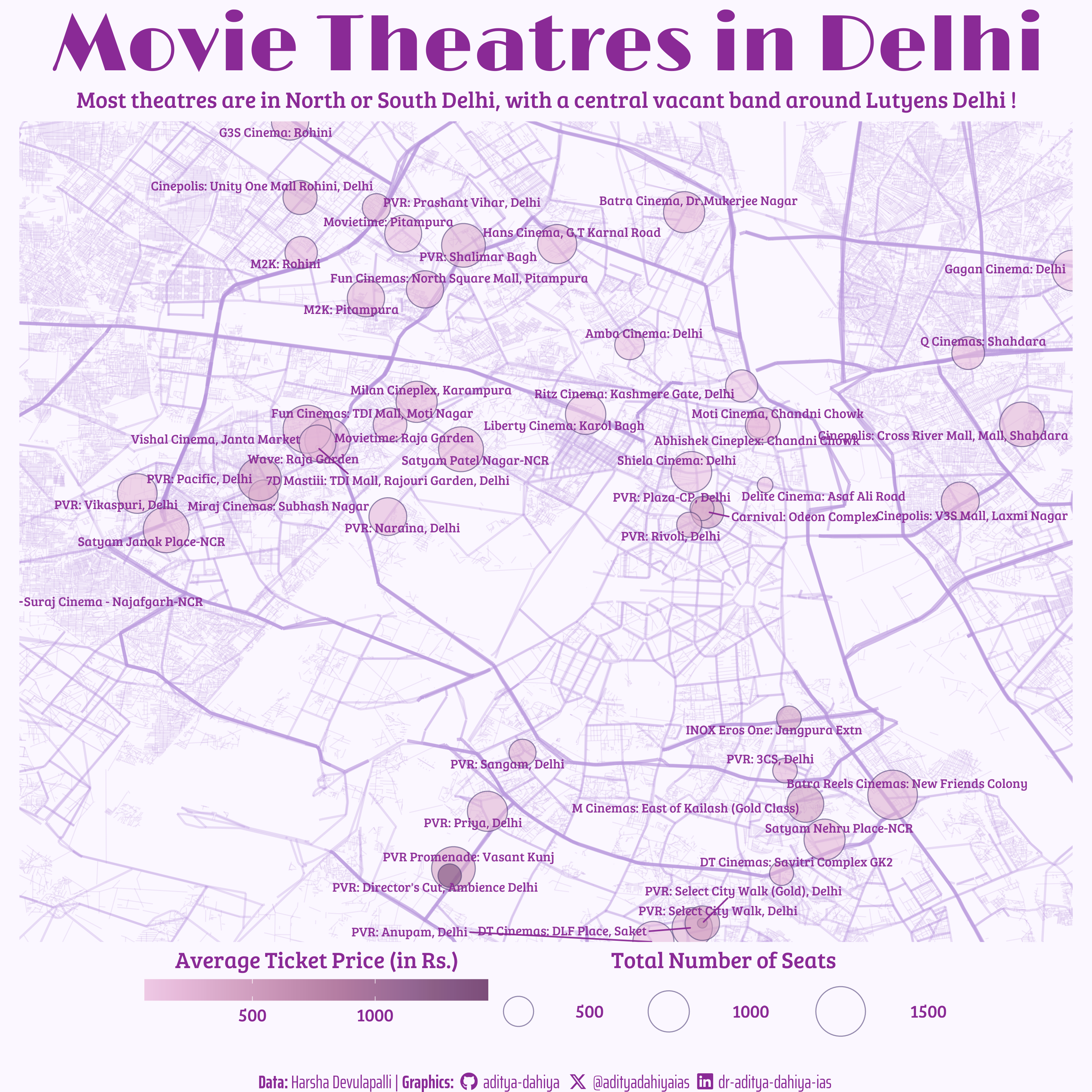
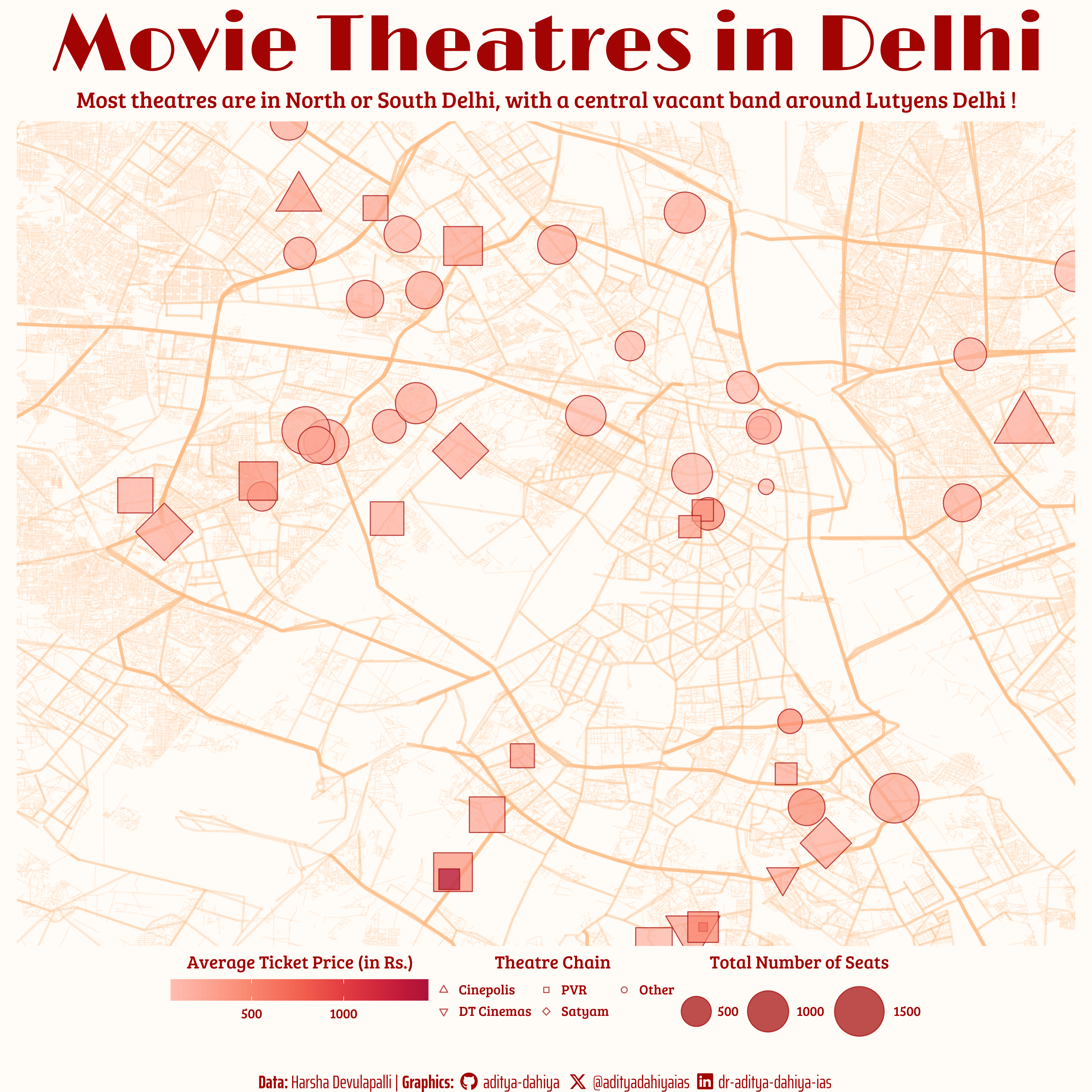
Let us customize the size and shape aesthetics in map of Delhi with Movie Theater Locations ( Figure 1 ), made in Chapter 11 (Section 11.7), and change the shapes, colours and sizes to produce Figure 2 .
Code
#==============================================================================#
# Library Load-in---------------------------------------------------------------
#==============================================================================#
library(tidyverse) # Data wrangling and plotting
library(osmdata) # Wrapper for Overpass API from Open Street Maps
library(janitor) # Cleaning names
library(sf) # For plotting maps
library(here) # Files location and loading
library(paletteer) # Lots of Color Palettes in R
library(colorspace) # Lightening and Darkening Colors
library(showtext) # Using Fonts More Easily in R Graphs
library(fontawesome) # Social Media icons
library(ggtext) # Markdown Text in ggplot2
library(patchwork) # For compiling plots
library(magick) # Work with Images and Logos
library(ggimage) # Background Image
#==============================================================================#
# Data Load-in------------------------------------------------------------------
#==============================================================================#
del_mov <- read_csv("https://raw.githubusercontent.com/HarshaDevulapalli/indian-movie-theatres/master/indian-movie-theatres.csv") |>
filter(city == "Delhi")
main_roads <- st_read(here::here("data",
"delhi_osm",
"delhi_main_roads.shp"))
st_crs(main_roads) <- "WGS 84"
minor_roads <- st_read(here::here("data",
"delhi_osm",
"delhi_minor_roads.shp"))
st_crs(minor_roads) <- "WGS 84"
very_minor_roads <- st_read(here::here("data",
"delhi_osm",
"delhi_veryminor_roads.shp"))
st_crs(very_minor_roads) <- "WGS 84"
#==============================================================================#
# Data Wrangling----------------------------------------------------------------
#==============================================================================#
coords <- del_mov |>
summarise(
top = max(lat),
bottom = min(lat),
left = min(lon),
right = max(lon)
) |>
as_vector()
# Adjust to remove the one leftmost (westward) cniema hall - outlier
percentage_removal_factor = 0.2
coords[3] <- coords[3] +
((coords[4] - coords[3]) * percentage_removal_factor)
# Impute average value to NAs
impute_na <- median(del_mov$average_ticket_price, na.rm = TRUE)
del_mov <- del_mov |>
mutate(average_ticket_price =
if_else(is.na(average_ticket_price),
impute_na,
average_ticket_price))
#==============================================================================#
# Options & Visualization Parameters--------------------------------------------
#==============================================================================#
# Load fonts
font_add_google("Limelight",
family = "title_font") # Font for titles
font_add_google("Saira Extra Condensed",
family = "caption_font") # Font for the caption
font_add_google("Bree Serif",
family = "body_font") # Font for plot text
showtext_auto()
# Colour Palette
mypal_c <- paletteer::scale_colour_paletteer_c("ggthemes::Purple")
mypal <- paletteer::paletteer_d("rcartocolor::Purp")
# Define colours
low_col <- mypal[4] # Low colour
hi_col <- mypal[6] # High colour
bg_col <- mypal[3] |> lighten(0.9) # Background Colour
text_col <- mypal[1] |> darken(0.6) # Colour for the text
text_hil <- mypal[6] |> darken(0.4) # Colour for the title
# Caption stuff
sysfonts::font_add(family = "Font Awesome 6 Brands",
regular = here::here("docs", "Font Awesome 6 Brands-Regular-400.otf"))
github <- ""
github_username <- "aditya-dahiya"
xtwitter <- ""
xtwitter_username <- "@adityadahiyaias"
linkedin <- ""
linkedin_username <- "dr-aditya-dahiya-ias"
social_caption <- glue::glue("<span style='font-family:\"Font Awesome 6 Brands\";'>{github};</span> <span style='color: {text_col}'>{github_username} </span> <span style='font-family:\"Font Awesome 6 Brands\";'>{xtwitter};</span> <span style='color: {text_col}'>{xtwitter_username}</span> <span style='font-family:\"Font Awesome 6 Brands\";'>{linkedin};</span> <span style='color: {text_col}'>{linkedin_username}</span>")
# Add text to plot--------------------------------------------------------------
plot_title <- "Movie Theatres in Delhi"
subtitle_text <- "Most theatres are in North or South Delhi, with a central vacant band around Lutyens Delhi !"
plot_subtitle <- paste(strwrap(subtitle_text, 100), collapse = "\n")
plot_caption <- paste0("**Data:** Harsha Devulapalli | ", "**Graphics:** ", social_caption)
#==============================================================================#
# Data Visualization------------------------------------------------------------
#==============================================================================#
g <- ggplot() +
geom_sf(
data =
main_roads |>
mutate(geometry = st_simplify(
geometry,
dTolerance = 50,
preserveTopology = TRUE)),
mapping = aes(geometry = geometry),
color = low_col,
linewidth = 1,
alpha = 0.4) +
geom_sf(
data =
minor_roads |>
mutate(geometry = st_simplify(
geometry,
dTolerance = 1,
preserveTopology = TRUE)),
color = low_col,
linewidth = 0.7,
alpha = 0.3) +
geom_sf(
data =
very_minor_roads |>
mutate(geometry = st_simplify(
geometry,
dTolerance = 10,
preserveTopology = TRUE)),
color = low_col,
linewidth = 0.3,
alpha = 0.2) +
geom_point(
data = del_mov,
mapping = aes(
x = lon,
y = lat,
size = total_seats,
fill = average_ticket_price
),
pch = 21,
color = text_hil,
alpha = 0.6
) +
ggrepel::geom_text_repel(
data = del_mov,
mapping = aes(
x = lon,
y = lat,
label = theatre_name
),
alpha = 0.95,
family = "body_font",
colour = text_col,
seed = 42,
size = 10,
segment.color = text_col
) +
coord_sf(
xlim = coords[c("left", "right")],
ylim = coords[c("bottom", "top")],
expand = FALSE) +
scale_fill_paletteer_c("ggthemes::Purple") +
scale_size_continuous(range = c(1, 15)) +
labs(title = plot_title,
subtitle = plot_subtitle,
caption = plot_caption,
fill = "Average Ticket Price (in Rs.)",
size = "Total Number of Seats") +
theme_void() +
guides(fill = guide_colorbar(title.position = "top",
barheight = unit(0.5, "cm"),
barwidth = unit(8, "cm")),
size = guide_legend(title.position = "top",
keywidth = unit(0.5, "cm"),
keyheight = unit(0.5, "cm"),
label.hjust = 0)) +
theme(
plot.caption = element_textbox(family = "caption_font",
hjust = 0.5,
colour = text_col,
size = unit(40, "cm")),
plot.title = element_text(hjust = 0.5,
size = unit(175, "cm"),
margin = margin(0.3,0,0.2,0,
unit = "cm"),
family = "title_font",
face = "bold",
colour = text_col),
plot.subtitle = element_text(hjust = 0.5,
size = unit(50, "cm"),
family = "body_font",
colour = text_col,
margin = margin(0,0,0.2,0,
unit = "cm")),
plot.background = element_rect(fill = bg_col,
color = bg_col,
linewidth = 0),
legend.position = "bottom",
legend.text = element_text(hjust = 0.5,
size = unit(40, "cm"),
family = "body_font",
colour = text_col),
legend.title = element_text(hjust = 0.5,
size = 50,
family = "body_font",
colour = text_col,
margin = margin(0,0,0,0)),
legend.box.margin = margin(0,0,0.5,0, unit = "cm"),
legend.box = "horizontal",
legend.spacing.y = unit(0.2, "cm")
)
#=============================================================================#
# Image Saving-----------------------------------------------------------------
#=============================================================================#
ggsave(
filename = here::here("docs", "delhimovies_tidy.png"),
plot = g,
device = "png",
dpi = "retina",
width = unit(10, "cm"),
height = unit(10, "cm"),
bg = bg_col
)
12.3 Line width & 12.4 Line type
The Figure 3 shows the use of custom scales in line-type and line-width as aesthetics.
Code
economics |>
  select(date, psavert, uempmed) |>
  pivot_longer(
    cols = c(psavert, uempmed),
    names_to = "indicator",
    values_to = "value"
  ) |>
  ggplot(aes(x = date,
             y = value,
             linetype = indicator,
             linewidth = indicator)) +
  geom_line() +
  scale_linetype_manual(
    values = c(1, 3),
    labels = c(
      "Personal savings rate (%)",
      "Median duration of unemployment, in weeks"
    ),
    name = NULL
  ) +
  scale_linewidth_manual(
    values = c(1, 0.5)
  ) +
  guides(
    linewidth = "none",
    linetype = guide_legend(
      override.aes = list(linewidth = 1),
      keywidth = unit(2, "cm")
    )
  ) +
  labs(
    x = NULL, y = NULL,
    title = "USA: Comparing Unemployment and Savings Rate trends"
  ) +
  cowplot::theme_half_open() +
  theme(
    legend.position = "bottom",
    axis.line = element_line(arrow = arrow(length = unit(3, "mm")))
  )