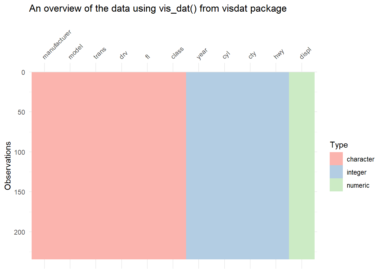
Chapter 2

First Steps

2.2.1 Exercises

Question 1

List five functions that you could use to get more information about the mpg dataset.

Here are the five functions for exploring the mpg dataset from the ggplot2 package in R, along with example code: –

1. Use str(mpg) to display the structure of the dataset mpg telling what is the class of each variable.

   Code

   str(mpg)

   tibble [234 × 11] (S3: tbl_df/tbl/data.frame)
    $ manufacturer: chr [1:234] "audi" "audi" "audi" "audi" ...
    $ model       : chr [1:234] "a4" "a4" "a4" "a4" ...
    $ displ       : num [1:234] 1.8 1.8 2 2 2.8 2.8 3.1 1.8 1.8 2 ...
    $ year        : int [1:234] 1999 1999 2008 2008 1999 1999 2008 1999 1999 2008 ...
    $ cyl         : int [1:234] 4 4 4 4 6 6 6 4 4 4 ...
    $ trans       : chr [1:234] "auto(l5)" "manual(m5)" "manual(m6)" "auto(av)" ...
    $ drv         : chr [1:234] "f" "f" "f" "f" ...
    $ cty         : int [1:234] 18 21 20 21 16 18 18 18 16 20 ...
    $ hwy         : int [1:234] 29 29 31 30 26 26 27 26 25 28 ...
    $ fl          : chr [1:234] "p" "p" "p" "p" ...
    $ class       : chr [1:234] "compact" "compact" "compact" "compact" ...

2. Employ glimpse(mpg) to obtain a concise overview of the dataset’s structure and its first few rows, offering a detailed glimpse of the data. It is similar to the previous function str()

   Code

   glimpse(mpg)

   Rows: 234
   Columns: 11
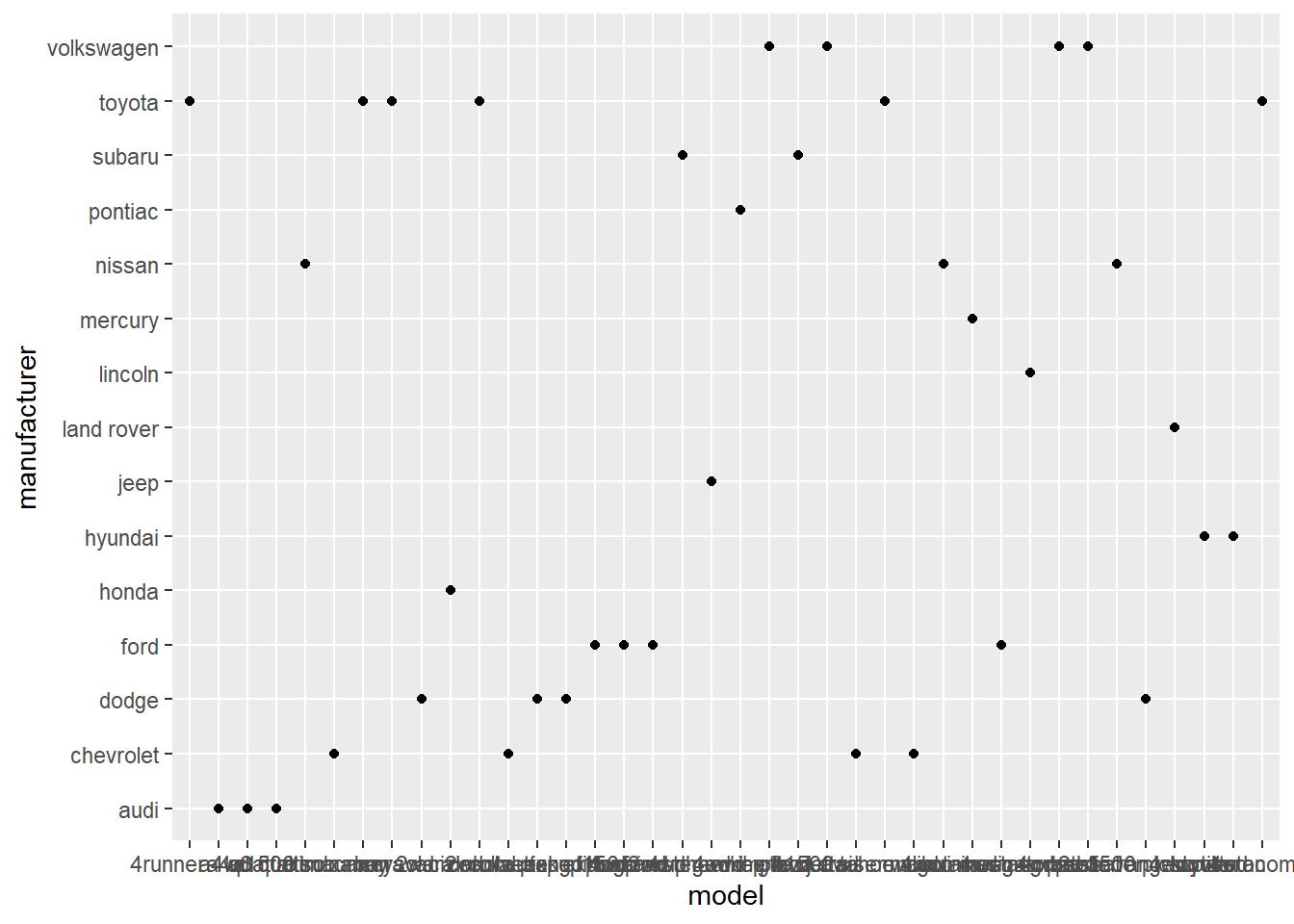
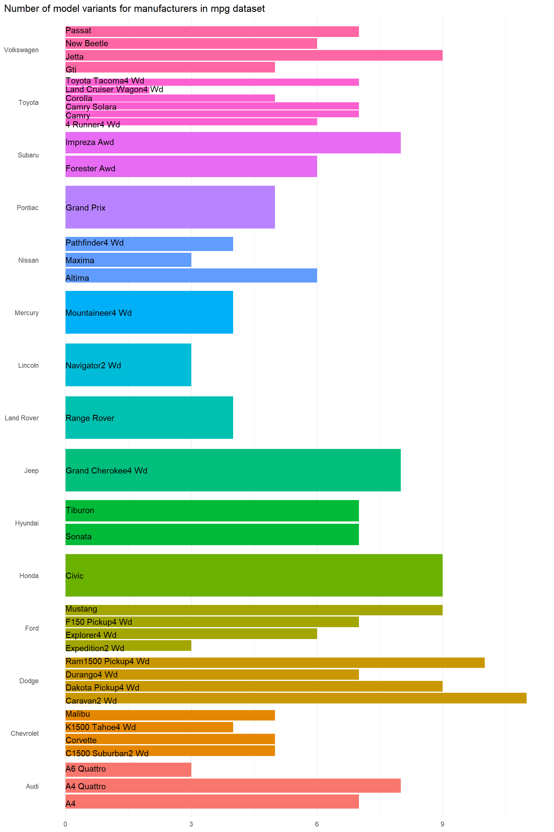
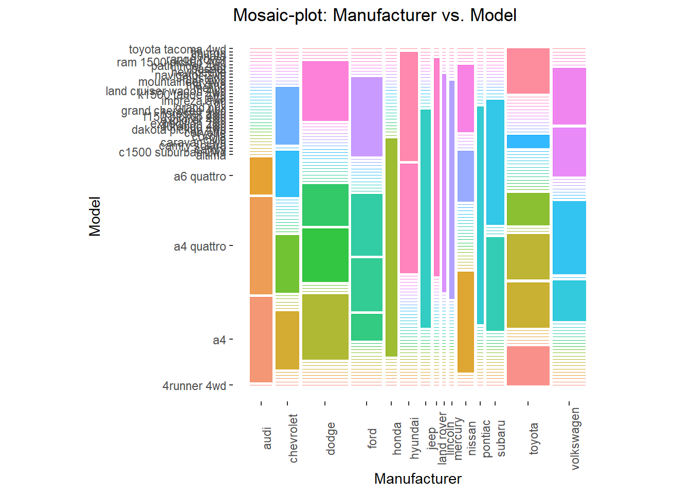
   $ manufacturer <chr> "audi", "audi", "audi", "audi", "audi", "audi", "audi", "…
   $ model        <chr> "a4", "a4", "a4", "a4", "a4", "a4", "a4", "a4 quattro", "…
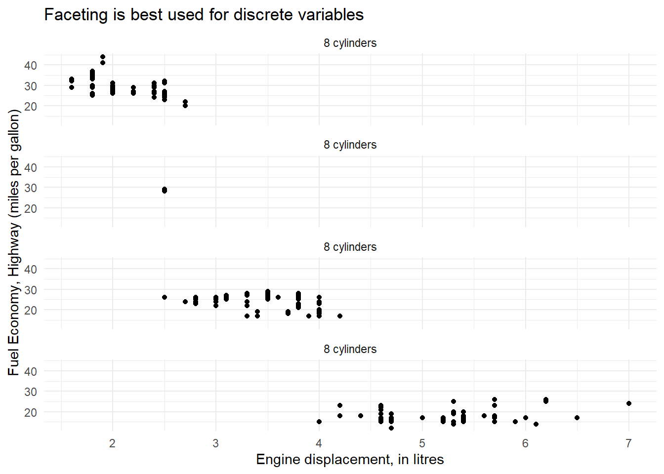
   $ displ        <dbl> 1.8, 1.8, 2.0, 2.0, 2.8, 2.8, 3.1, 1.8, 1.8, 2.0, 2.0, 2.…
   $ year         <int> 1999, 1999, 2008, 2008, 1999, 1999, 2008, 1999, 1999, 200…
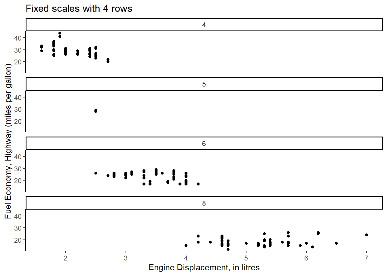
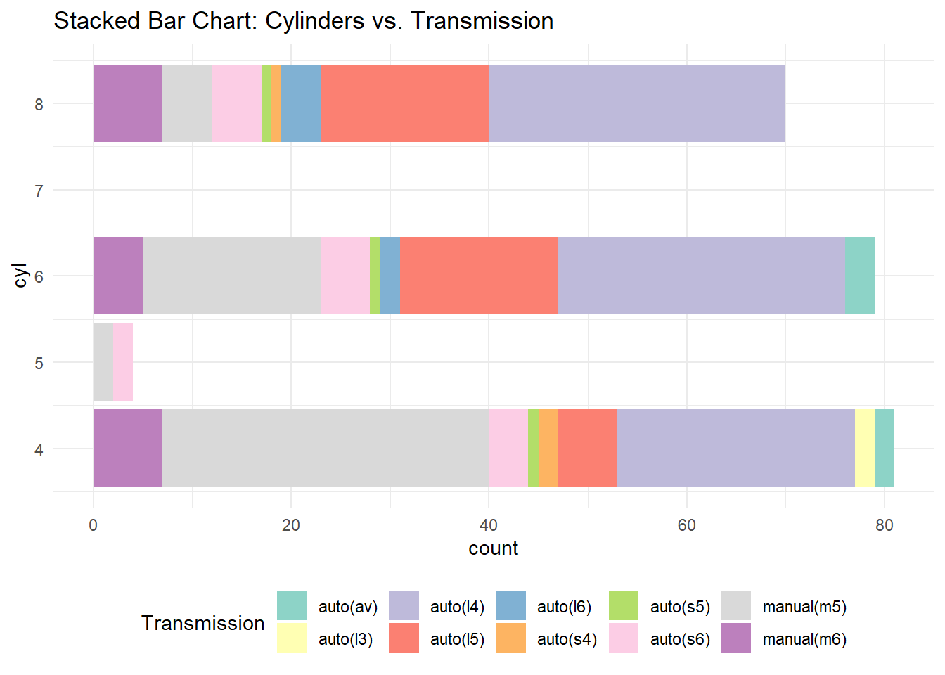
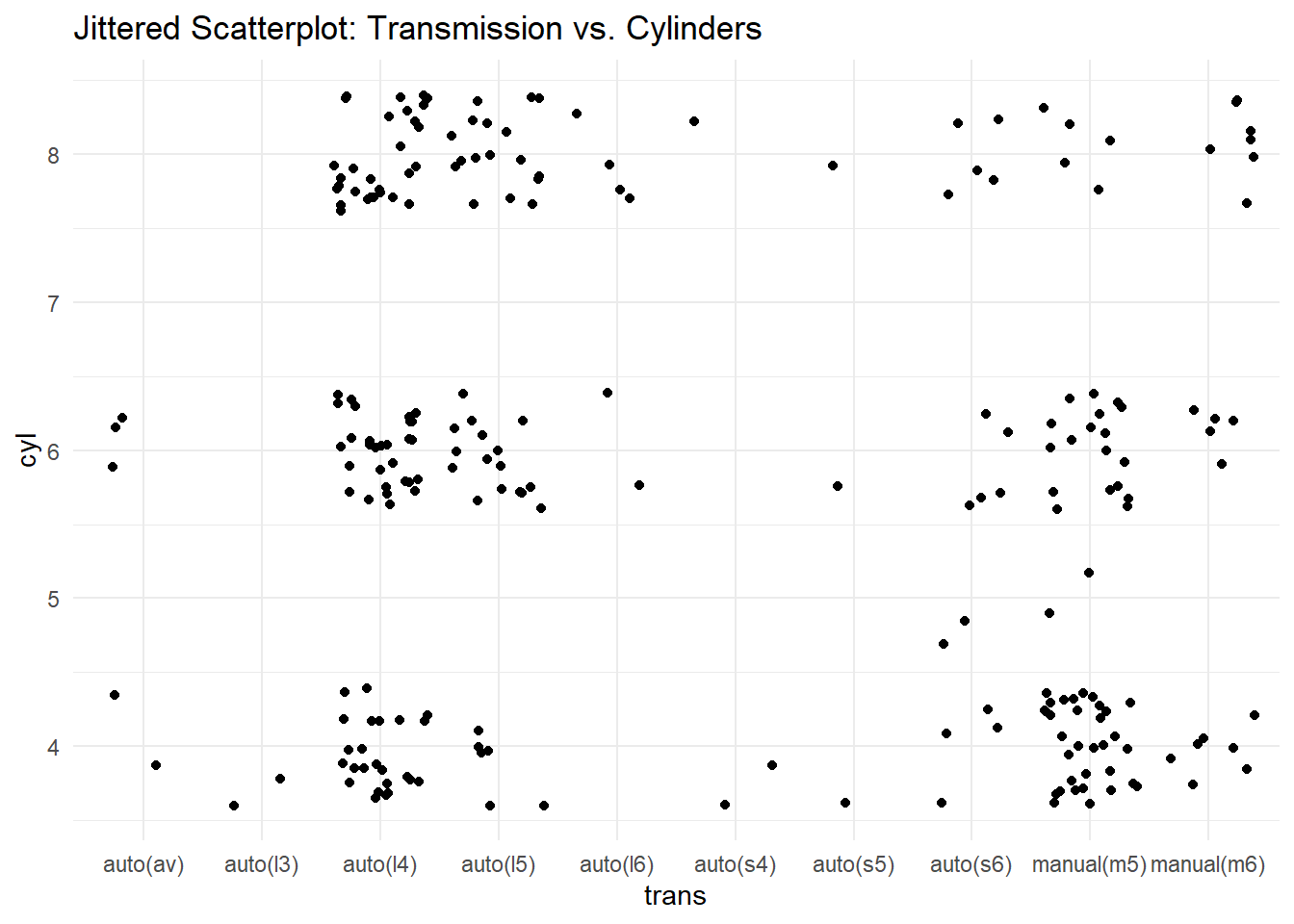
   $ cyl          <int> 4, 4, 4, 4, 6, 6, 6, 4, 4, 4, 4, 6, 6, 6, 6, 6, 6, 8, 8, …
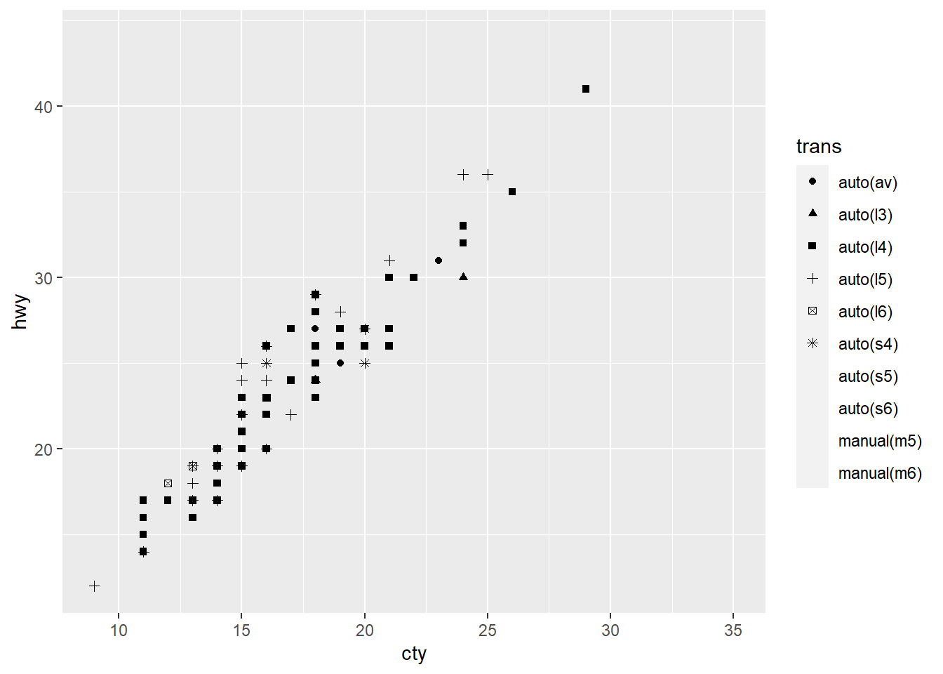
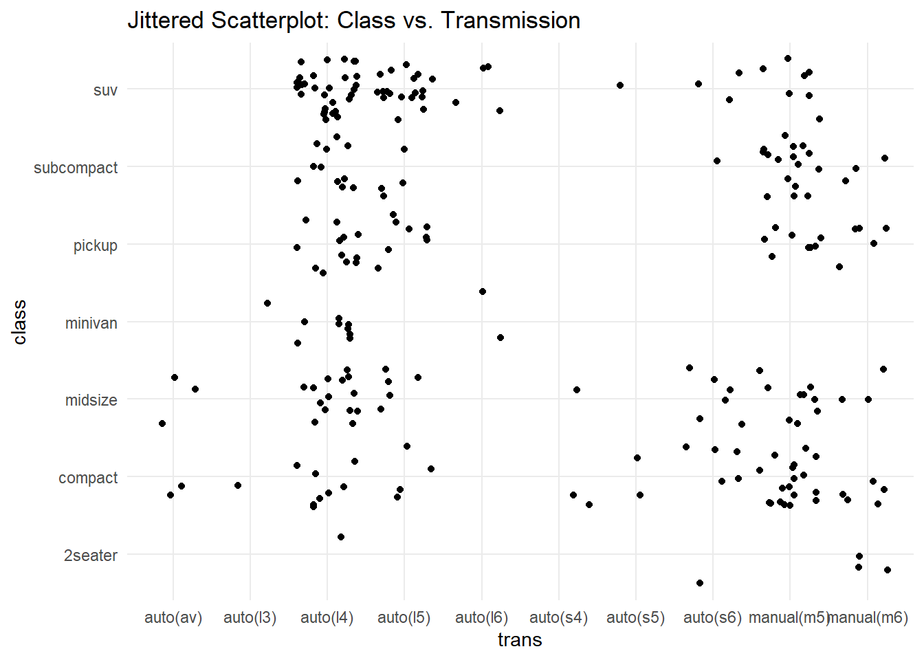
   $ trans        <chr> "auto(l5)", "manual(m5)", "manual(m6)", "auto(av)", "auto…
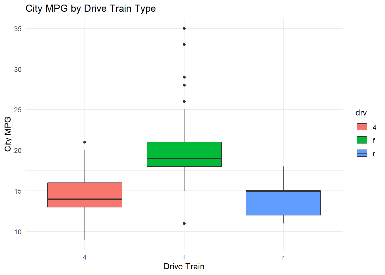
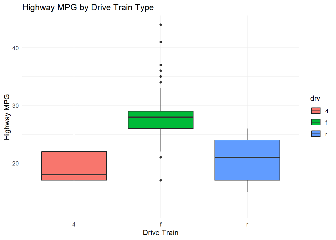
   $ drv          <chr> "f", "f", "f", "f", "f", "f", "f", "4", "4", "4", "4", "4…
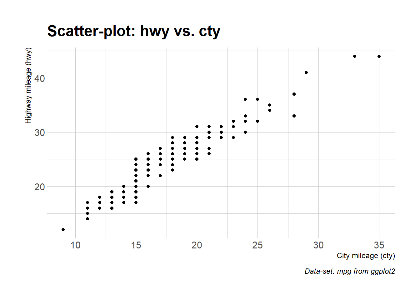
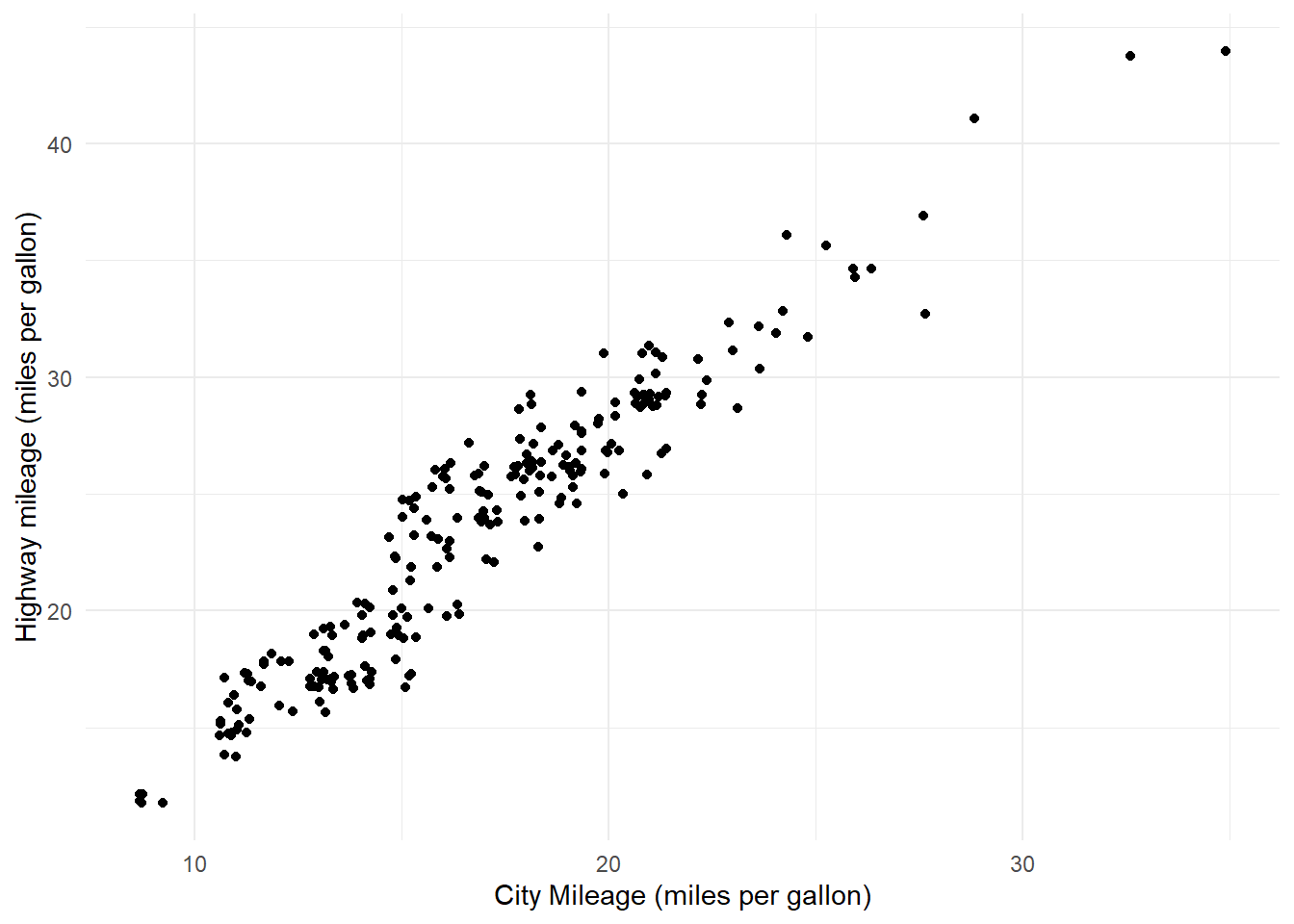
   $ cty          <int> 18, 21, 20, 21, 16, 18, 18, 18, 16, 20, 19, 15, 17, 17, 1…
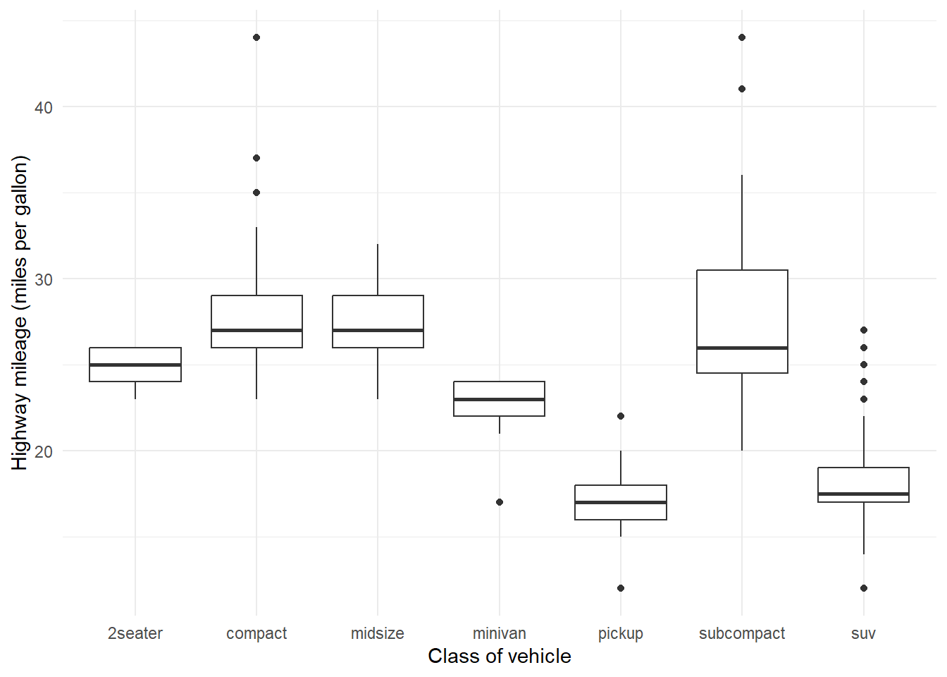
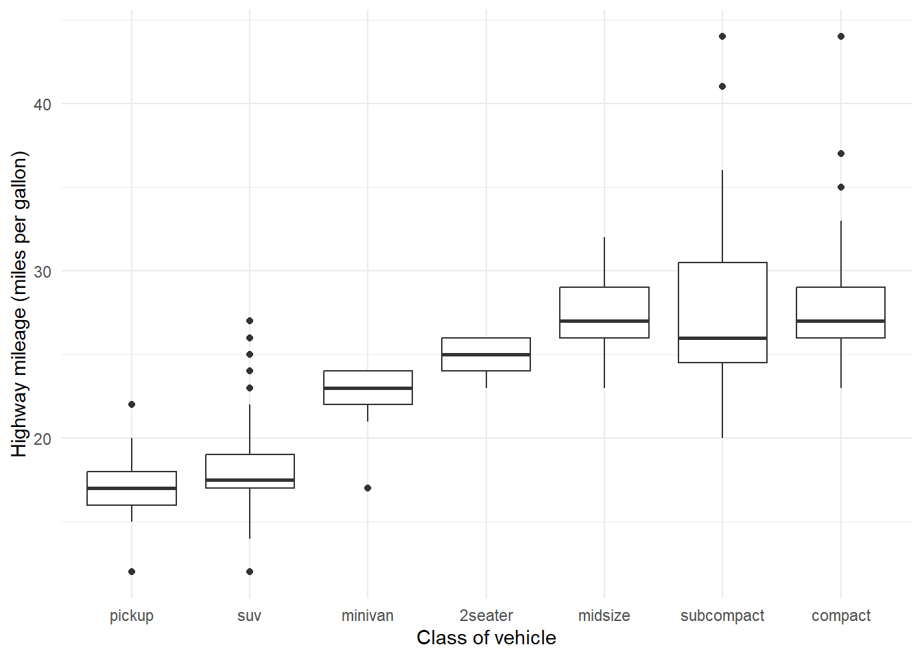
   $ hwy          <int> 29, 29, 31, 30, 26, 26, 27, 26, 25, 28, 27, 25, 25, 25, 2…
   $ fl           <chr> "p", "p", "p", "p", "p", "p", "p", "p", "p", "p", "p", "p…
   $ class        <chr> "compact", "compact", "compact", "compact", "compact", "c…

3. Run summary(mpg) to generate a statistical summary of the variables within the mpg dataset, providing measures like mean, median, and quartiles.

   Code

   summary(mpg)

    manufacturer          model               displ            year     
    Length:234         Length:234         Min.   :1.600   Min.   :1999  
    Class :character   Class :character   1st Qu.:2.400   1st Qu.:1999  
    Mode  :character   Mode  :character   Median :3.300   Median :2004  
                                          Mean   :3.472   Mean   :2004  
                                          3rd Qu.:4.600   3rd Qu.:2008  
                                          Max.   :7.000   Max.   :2008  
         cyl           trans               drv                 cty       
    Min.   :4.000   Length:234         Length:234         Min.   : 9.00  
    1st Qu.:4.000   Class :character   Class :character   1st Qu.:14.00  
    Median :6.000   Mode  :character   Mode  :character   Median :17.00  
    Mean   :5.889                                         Mean   :16.86  
    3rd Qu.:8.000                                         3rd Qu.:19.00  
    Max.   :8.000                                         Max.   :35.00  
         hwy             fl               class          
    Min.   :12.00   Length:234         Length:234        
    1st Qu.:18.00   Class :character   Class :character  
    Median :24.00   Mode  :character   Mode  :character  
    Mean   :23.44                                        
    3rd Qu.:27.00                                        
    Max.   :44.00                                        

4. Utilize dfSummary(mpg) from the summarytools package to obtain a comprehensive summary report with various statistics and visualizations for the mpg dataset.

   Code

   library(summarytools)
   st_options(plain.ascii = FALSE)
   print(
     summarytools::dfSummary(mpg,
                           plain.ascii = FALSE,
                           headings = FALSE,
                           display.labels = FALSE,
                           silent = TRUE),
     method = "render")

   No	Variable	Stats / Values	Freqs (% of Valid)	Graph	Valid	Missing
   1	manufacturer [character]	1. dodge 2. toyota 3. volkswagen 4. ford 5. chevrolet 6. audi 7. hyundai 8. subaru 9. nissan 10. honda [ 5 others ]	37 ( 15.8% ) 34 ( 14.5% ) 27 ( 11.5% ) 25 ( 10.7% ) 19 ( 8.1% ) 18 ( 7.7% ) 14 ( 6.0% ) 14 ( 6.0% ) 13 ( 5.6% ) 9 ( 3.8% ) 24 ( 10.3% )		234 (100.0%)	0 (0.0%)
   2	model [character]	1. caravan 2wd 2. ram 1500 pickup 4wd 3. civic 4. dakota pickup 4wd 5. jetta 6. mustang 7. a4 quattro 8. grand cherokee 4wd 9. impreza awd 10. a4 [ 28 others ]	11 ( 4.7% ) 10 ( 4.3% ) 9 ( 3.8% ) 9 ( 3.8% ) 9 ( 3.8% ) 9 ( 3.8% ) 8 ( 3.4% ) 8 ( 3.4% ) 8 ( 3.4% ) 7 ( 3.0% ) 146 ( 62.4% )		234 (100.0%)	0 (0.0%)
   3	displ [numeric]	Mean (sd) : 3.5 (1.3) min ≤ med ≤ max: 1.6 ≤ 3.3 ≤ 7 IQR (CV) : 2.2 (0.4)	35 distinct values		234 (100.0%)	0 (0.0%)
   4	year [integer]	Min : 1999 Mean : 2003.5 Max : 2008	1999 : 117 ( 50.0% ) 2008 : 117 ( 50.0% )		234 (100.0%)	0 (0.0%)
   5	cyl [integer]	Mean (sd) : 5.9 (1.6) min ≤ med ≤ max: 4 ≤ 6 ≤ 8 IQR (CV) : 4 (0.3)	4 : 81 ( 34.6% ) 5 : 4 ( 1.7% ) 6 : 79 ( 33.8% ) 8 : 70 ( 29.9% )		234 (100.0%)	0 (0.0%)
   6	trans [character]	1. auto(av) 2. auto(l3) 3. auto(l4) 4. auto(l5) 5. auto(l6) 6. auto(s4) 7. auto(s5) 8. auto(s6) 9. manual(m5) 10. manual(m6)	5 ( 2.1% ) 2 ( 0.9% ) 83 ( 35.5% ) 39 ( 16.7% ) 6 ( 2.6% ) 3 ( 1.3% ) 3 ( 1.3% ) 16 ( 6.8% ) 58 ( 24.8% ) 19 ( 8.1% )		234 (100.0%)	0 (0.0%)
   7	drv [character]	1. 4 2. f 3. r	103 ( 44.0% ) 106 ( 45.3% ) 25 ( 10.7% )		234 (100.0%)	0 (0.0%)
   8	cty [integer]	Mean (sd) : 16.9 (4.3) min ≤ med ≤ max: 9 ≤ 17 ≤ 35 IQR (CV) : 5 (0.3)	21 distinct values		234 (100.0%)	0 (0.0%)
   9	hwy [integer]	Mean (sd) : 23.4 (6) min ≤ med ≤ max: 12 ≤ 24 ≤ 44 IQR (CV) : 9 (0.3)	27 distinct values		234 (100.0%)	0 (0.0%)
   10	fl [character]	1. c 2. d 3. e 4. p 5. r	1 ( 0.4% ) 5 ( 2.1% ) 8 ( 3.4% ) 52 ( 22.2% ) 168 ( 71.8% )		234 (100.0%)	0 (0.0%)
   11	class [character]	1. 2seater 2. compact 3. midsize 4. minivan 5. pickup 6. subcompact 7. suv	5 ( 2.1% ) 47 ( 20.1% ) 41 ( 17.5% ) 11 ( 4.7% ) 33 ( 14.1% ) 35 ( 15.0% ) 62 ( 26.5% )		234 (100.0%)	0 (0.0%)

   Generated by summarytools 1.0.1 (R version 4.3.1)
   2023-10-23

5. Enhance data exploration with vis_dat(mpg) from the visdat package, which offers interactive visualizations to better understand the data-set’s contents and identify missing values.

   Code

   library(visdat)
   
   visdat::vis_dat(mpg) + scale_fill_brewer(palette = "Pastel1") +
     labs(title = "An overview of the data using vis_dat() from visdat package")

   

Question 2

How can you find out what other datasets are included with ggplot2?

To find out what datasets are included with the ggplot2 package, you can use the data() function. You can use the data() function to list all the datasets available in the ggplot2 package.

Code

data(package = "ggplot2")

Question 3

Apart from the US, most countries use fuel consumption (fuel consumed over fixed distance) rather than fuel economy (distance travelled with fixed amount of fuel). How could you convert cty and hwy into the European standard of l/100km?

In the R formula, we convert miles per gallon (mpg) to liters per 100 kilometers (L/100km). The conversion factor, 235.21, is used to perform the conversion. To convert mpg to L/100km, we divide the conversion factor by the mpg value.

\[ \text{L/100km} = \frac{235.21}{\text{mpg}} \tag{1}\] The conversion factor of 235.21 is derived from the following logic:

1. 1 mile is equal to approximately 1.609 kilometers.
2. 1 gallon is equal to approximately 3.785 liters.

To convert from miles per gallon (mpg) to liters per 100 kilometers (L/100km), we need to reverse the units. So, we divide the number of miles (1 mile) by the number of gallons (1 gallon) to get the number of kilometers per liter. This can be expressed as:

\[ \text{Kilometers per Liter} = \frac{1 \text{ mile}}{1 \text{ gallon}} \times \frac{1.609 \text{ kilometers}}{1 \text{ mile}} \times \frac{1 \text{ liter}}{3.785 \text{ gallons}} \approx 0.4251 \text{ kilometers per liter} \tag{2}\]

Now, to express fuel efficiency in liters per 100 kilometers, we need to scale up by 100:

\[ \text{L/100km} = \frac{1}{0.4251} \times 100 \approx 235.21 \text{ L/100km per 1 kilometer per liter} \tag{3}\]

So, when you divide 235.21 by miles per gallon (mpg), you are effectively converting from miles per gallon to liters per 100 kilometers, accounting for the differences in units and scaling by 100 to express the consumption over a distance of 100 kilometers.

Now, you can include the R code and LaTeX explanation in an R Markdown document for a more structured presentation. When you knit the R Markdown document, it will generate a formatted document with both the code and explanations.

Code

# Conversion factor from mpg to L/100km
conversion_factor <- 235.21

mpg |> 
  mutate(
    cty = conversion_factor/cty,
    hwy = conversion_factor/hwy
  ) |> 
  slice_head(n = 5) |> 
  gt() |> gtExtras::gt_theme_538() |> 
  fmt_number(columns = cty:hwy,
             decimals = 2)

Table 1:

mpg dataset with mileage in Liters per 100 km

manufacturer	model	displ	year	cyl	trans	drv	cty	hwy	fl	class
audi	a4	1.8	1999	4	auto(l5)	f	13.07	8.11	p	compact
audi	a4	1.8	1999	4	manual(m5)	f	11.20	8.11	p	compact
audi	a4	2.0	2008	4	manual(m6)	f	11.76	7.59	p	compact
audi	a4	2.0	2008	4	auto(av)	f	11.20	7.84	p	compact
audi	a4	2.8	1999	6	auto(l5)	f	14.70	9.05	p	compact

Question 4

Which manufacturer has the most models in this dataset? Which model has the most variations? Does your answer change if you remove the redundant specification of drive train (e.g. “pathfinder 4wd”, “a4 quattro”) from the model name?

As we can see below in Table 2, Toyota has the most models in the data-set.

Code

# Group 'mpg' data by 'manufacturer.'
mpg |> 
  group_by(manufacturer) |> 

  # Count distinct 'model' values for each manufacturer.
  summarize(models = n_distinct(model)) |> 

  # Sort in descending order based on 'n_models.'
  arrange(desc(models)) |> 
  
  # Select the top 5 manufacturers.
  slice_head(n = 5) |> 
  
  # Create a table and apply a specific theme to it.
  gt() |> gt_theme_538()

Table 2:

Top 5 manufacturers in mpg data-set as per number of models

manufacturer	models
toyota	6
chevrolet	4
dodge	4
ford	4
volkswagen	4

And, as we can see in the Table 3 below, the Dodge Caravan (2 wheel drive) model has the most variations, i.e., 11 in number.

Code

mpg |> 
  count(manufacturer, model, sort = TRUE) |> 
  slice_head(n = 5) |> 
  rename(variations = n) |> 
  gt() |> gt_theme_538()

Table 3:

Number of variations in the different models of cars - top 5

manufacturer	model	variations
dodge	caravan 2wd	11
dodge	ram 1500 pickup 4wd	10
dodge	dakota pickup 4wd	9
ford	mustang	9
honda	civic	9

2.3.1 Exercises

Question 1

How would you describe the relationship between cty and hwy? Do you have any concerns about drawing conclusions from that plot?

There is a positive correlation between cty and hwy , as shown in Figure 1. However, one concern we have is whether this correlation is causative in nature, or is it a direct correlation, or is it caused by a third unknown variable, i.e. confounding.

Confounding is a distortion of the association between independent and dependent variables. It occurs when a third variable is independently associated with both. This can happen when the primary exposure of interest is mixed up with some other factor that is associated with the outcome.

For example, perhaps it is the engine displacement that determines both city and highway mileage, and both have a common link, rather than a direct association.

Note: I am using theme_ipsum() from the hrbrthemes package (Rudis 2020).

Code

mpg |> 
  ggplot(aes(x = cty, y = hwy)) +
  geom_point() +
  labs(x = "City mileage (cty)", 
       y = "Highway mileage (hwy)",
       title = "Scatter-plot: hwy vs. cty",
       caption = "Data-set: mpg from ggplot2") +
  hrbrthemes::theme_ipsum()

Figure 1: A Scatter-plot of city and highway milea for the mpg dataset

Question 2

What does ggplot(mpg, aes(model, manufacturer)) + geom_point() show? Is it useful? How could you modify the data to make it more informative?

The code ggplot(mpg, aes(model, manufacturer)) + geom_point() is used to create a scatter plot, where the mpg dataset is being used, and it’s mapping the model variable to the x-axis and the manufacturer variable to the y-axis. The geom_point() function is responsible for adding points to the plot.

Code

ggplot(mpg, aes(model, manufacturer)) + geom_point()

Figure 2: Plot produced by the code given in Question 2

Here’s a detailed explanation of why this code and its resulting Figure 2 isn’t useful:

1. Data Mapping:

   • model is mapped to the x-axis: The car models don’t have a specific order, i.e. it is a categorical variable, not an ordinal or continuous variable.
   • manufacturer is mapped to the y-axis: Again, manufacturer is a categorical variable with no specific order. Thus, representing it on y-axis is not advisable.

2. Visualization:

   • The plot will consist of multiple points where each point represents a combination of a car model and its manufacturer. As, we can expect, each observation will have a unique model. There is no specific information or pattern being displayed as scatter plot doesn’t connect the points.
   • The plot suffers from over-plotting if there are many data points when a single model has many variants (alpha aesthetic has not been defined here). Further, since each unique model and manufacturer combination will be displayed as a separate point, it is difficult to discern patterns or relationships.
   • Thus, this plot has very limited usefulness is identifying trends or make specific insights.

Modifications for More Informativeness: To make the plot more informative, you can consider the following modifications:

1. Changing the plot geom: If our purpose is to show the number of model variants for each manufacturer, we might shift to a bar plot, with faceting on the manufacturer as shown in Figure 3 .

   Code

   mpg |> 
   
     # Counting number of variants for each model
     count(manufacturer, model) |> 
   
     # Nicer looking names
     mutate(manufacturer = snakecase::to_title_case(manufacturer),
            model = snakecase::to_title_case(model, numerals = "left")) |> 
   
     # Plot
     ggplot(aes(x = n, 
                y = manufacturer,
                group = model, 
                fill = manufacturer)) +
   
     # Grouped bar chart
     geom_bar(position = "dodge2",
              stat = "identity") +
   
     # Adding names of models
     geom_text(aes(label = model,
                   x = 0),
               position = position_dodge2(width = 1),
               hjust = "left") +
     theme_minimal() +
     theme(panel.grid.major.y = element_blank(),
           legend.position = "none",
           plot.title.position = "plot") +
     labs(y = NULL, x = NULL,
          title = "Number of model variants for manufacturers in mpg dataset")

   

   Figure 3: Grouped horizontal bar plot showing number of variants for different car models in mpg dataset

2. Labels, Title, Color and Size Aesthetics: If we insist on using the same plot as given in the question, we can use additional aesthetics like color or point size to encode more information. For instance, you could use color to represent a third variable, such as “class” (economy, midsize, compact, etc.), and point size to represent another variable, like “displacement.” We can further sort the manufacturers and models alphabetically.

   Code

   # Create some factors to order the manufacturers and model names in a specific order
   man_lev <- mpg |> 
     distinct(manufacturer) |> pull(manufacturer)
   
   mod_lev <- mpg |> 
     group_by(manufacturer) |> 
     arrange(manufacturer, model) |> pull(model) |> unique()
   
   # Start the plot
   mpg |> 
   
     # reorder the manufacturers by alphabetically and models by numbers
       mutate(
       manufacturer = fct(manufacturer, levels = man_lev),
       model = fct(model, levels = mod_lev)
     ) |> 
   
     # Create the same scatter plot, adding size and color aesthetic
       ggplot(aes(x = model,
                y = manufacturer,
                size = displ,
                col = manufacturer)) +
   
     # A geom_jitter instead of geom_point to avoid overlap of variants of a model
     geom_jitter(alpha = 0.3,
                 width = 0,
                 height = 1) +
   
     # Plot beautification and customization
   
     labs(x = NULL, y = NULL) +
     theme_minimal() +
     theme(legend.position = "none",
           panel.grid.minor.x = element_blank(),
           panel.grid.major.x = element_blank(),
           axis.text.x = element_text(angle = 90, 
                                      hjust = 1,
                                      vjust = 0.5))

   

   Figure 4: Adding other informative aesthetics to the points in given plot

These modifications can help you gain more insight from your data and make your visualization more informative. The choice of modifications should depend on the specific questions you want to answer and the nature of your dataset.

Question 3

Describe the data, aesthetic mappings and layers used for each of the following plots. You’ll need to guess a little because you haven’t seen all the datasets and functions yet, but use your common sense! See if you can predict what the plot will look like before running the code.

1. ggplot(mpg, aes(cty, hwy)) + geom_point()

2. ggplot(diamonds, aes(carat, price)) + geom_point()

3. ggplot(economics, aes(date, unemploy)) + geom_line()

4. ggplot(mpg, aes(cty)) + geom_histogram()

Let’s break down each of the provided ggplot2 code snippets and describe the data, aesthetic mappings, and layers used for the plots:

1. ggplot(mpg, aes(cty, hwy)) + geom_point()
   • Data: The data for this plot comes from the ‘mpg’ dataset, which is typically included in the ggplot2 package. This dataset contains information about the fuel efficiency of various car models.
   • Aesthetic Mappings: It uses aesthetic mappings to represent the ‘cty’ (city miles per gallon) variable on the x-axis and the ‘hwy’ (highway miles per gallon) variable on the y-axis.
   • Layers: This plot consists of a single layer represented by geom_point(), which adds points to the plot, creating a scatter plot of ‘cty’ against ‘hwy’.
2. ggplot(diamonds, aes(carat, price)) + geom_point()
   • Data: The data for this plot comes from the ‘diamonds’ dataset, another built-in dataset in ggplot2, containing information about diamonds, including their carat weight and price.
   • Aesthetic Mappings: It uses aesthetic mappings to represent the ‘carat’ variable on the x-axis and the ‘price’ variable on the y-axis.
   • Layers: This plot also consists of a single layer represented by geom_point(), which adds points to the plot, creating a scatter plot of diamond carat weight against their prices.
3. ggplot(economics, aes(date, unemploy)) + geom_line()
   • Data: The data for this plot comes from the ‘economics’ dataset, which is included in the ggplot2 package. This dataset contains economic data, including the ‘date’ and ‘unemploy’ (number of unemployed individuals) variables.
   • Aesthetic Mappings: It uses aesthetic mappings to represent the ‘date’ variable on the x-axis and the ‘unemploy’ variable on the y-axis.
   • Layers: This plot consists of a single layer represented by geom_line(), which connects points with lines, creating a time series line plot of the number of unemployed individuals over time.
4. ggplot(mpg, aes(cty)) + geom_histogram()
   • Data: The data for this plot also comes from the ‘mpg’ dataset.
   • Aesthetic Mappings: It uses an aesthetic mapping to represent only the ‘cty’ variable, which will be plotted on the x-axis. Since it’s a histogram, the y-axis represents the count of observations in each bin.
   • Layers: This plot consists of a single layer represented by geom_histogram(), which creates a histogram of the cty variable, showing the distribution of city miles per gallon in the dataset.

Each of these plots uses different datasets and aesthetic mappings, and they employ different types of geoms (layers) to represent the data in various ways, such as scatter plots, line plots, and histograms, depending on the specific data and the analysis or visualization goals.

2.4.1 Exercises

Question 1

Experiment with the colour, shape and size aesthetics. What happens when you map them to continuous values? What about categorical values? What happens when you use more than one aesthetic in a plot?

We can experiment with the colour, shape, and size aesthetics using both continuous and categorical variables in the mpg dataset. Figure 5 shows six separate scatter plots using different combinations of colour, shape, and size aesthetics, with both continuous and categorical variables: –

Code

# Create a ggplot2 plot with 'mpg' dataset
p <- ggplot(mpg, aes(x = cty, y = hwy)) + theme_minimal()

# Continuous variable with color, shape, and size aesthetics
p + geom_point(aes(color = displ))
  
p + geom_text(aes(x = 20, y = 30),
    label = "Error: Shape aesthetic does not \nwork with a continuous variable")

p + geom_point(aes(size = displ), alpha = 0.2)

# Categorical variable with color, shape, and size aesthetics
p + geom_point(aes(color = factor(class)))

p + geom_point(aes(shape = factor(class)))

p + geom_point(aes(size = factor(class)), alpha = 0.2)

(a) Continuous Variable with Color Aesthetic

(b) Continuous Variable with Shape Aesthetic

(c) Continuous Variable with Size Aesthetic

(d) Categorical Variable with Color Aesthetic

(e) Categorical Variable with Shape Aesthetic

(f) Categorical Variable with Size Aesthetic

Figure 5: Using continuous and categorical variables on the three aesthetics - colour, shape and size

Insights:

• size aesthetic works well with continuous variable (or, at worse, an ordinal variable). It should not be used with categorical variable.

• shape aesthetic works only with categorical variable. It simply does not work with a continuous variable.

• color works well with categorical and continuous variables.

When you use more than one aesthetic in a plot, you can create a plot that contains multiple layers of information, with each aesthetic conveying a different aspect of the data. While this can provide a rich and detailed representation of your data, it can also lead to a plot that becomes too complex and difficult to perceive for several reasons:

1. Clutter: Multiple aesthetics, such as color, shape, size, and others, can lead to visual clutter, especially when you have a large dataset. This can make it challenging for viewers to discern patterns and relationships within the data.

2. Cognitive Overload: When a plot contains too many aesthetics, viewers may struggle to process the information efficiently. It requires more cognitive effort to interpret the various aesthetic mappings, leading to information overload.

3. Reduced Clarity: Complex plots can reduce the clarity and simplicity that is often desirable in data visualization. Clutter and complexity can obscure the main message you want to convey, making it harder for the audience to understand the key insights.

4. Color Confusion: Overusing color can be particularly problematic. If multiple categories or variables are assigned distinct colors, it can be challenging to differentiate between them, especially if some colors are similar or hard to distinguish.

5. Interference: When multiple aesthetics are used, there’s a potential for interference or overlap between different visual elements. For example, if you use both color and size aesthetics, larger points with different colors may overlap, making it challenging to discern individual points.

6. Ineffectiveness: Sometimes, adding multiple aesthetics may not actually enhance the plot’s effectiveness or communicative power. Instead, it might complicate the plot without providing significant additional insights.

To avoid making a plot too complex and difficult to perceive, it’s essential to carefully consider the goals of your visualization and the message you want to convey. It’s often better to use a limited number of aesthetics thoughtfully, or using faceting.

Question 2

What happens if you map a continuous variable to shape? Why? What happens if you map trans to shape? Why?

Mapping a continuous variable to the shape aesthetic in ggplot2, it throws up an error, because, the shape aesthetic is designed for categorical variables, not continuous ones. When you attempt to deliberately map a continuous variable to shape, ggplot2 will, at best, treat it as a categorical variable, which can lead to unintended and potentially confusing results.

Let’s consider both scenarios using the mpg dataset:

1. Mapping a Continuous Variable (e.g., displ) to Shape Aesthetic:

   ggplot(mpg, aes(x = cty, y = hwy, shape = displ)) + geom_point()
   
   # Error in `geom_point()`:
   # ! Problem while computing aesthetics.
   # ℹ Error occurred in the 1st layer.
   # Caused by error in `scale_f()`:
   # ! A continuous variable cannot be mapped to the shape aesthetic
   # ℹ choose a different aesthetic or use `scale_shape_binned()`
   # Run `rlang::last_trace()` to see where the error occurred.

   When you map a continuous variable like displ (engine displacement) to the shape aesthetic, ggplot2 will treat each unique value of ‘displ’ as a separate category and assign a different shape to each value. This can result in a plot with many unique shapes, which can be difficult to interpret. Thus, ggplot2 throws up an error. The shapes do not have any inherent order or meaning in this context, so the plot may not provide clear insights.

2. Mapping a Categorical Variable (e.g., trans) to Shape:

   Code

   ggplot(mpg, aes(x = cty, y = hwy, shape = trans)) + geom_point()

   

   Figure 6: Mapping a Categorical Variable: Transmission (trans) to Shape aesthetic

   When you map a categorical variable like ‘trans’ (transmission type) to the shape aesthetic, ggplot2 assigns a unique shape to each category in the ‘trans’ variable. However, there are a limited number of shapes in ggplot2 and thus many shapes (like auto(s5) , auto(s6) , manual(m5) and manual(m6) ) go un-plotted thus leading to missing data. In any case, it is generally not advisable to plot more than 4-5 shapes in a plot to keep it nice and simple.

In summary, mapping a continuous variable to the shape aesthetic may not be possible. However, mapping a categorical variable to shape can be useful, provided the number of categories is not too much.

Question 3

How is drive train related to fuel economy? How is drive train related to engine size and class?

To understand the relationship between drive train, fuel economy, engine size, and class in the mpg dataset, you can create a series of plots. We’ll use scatter plots and bar plots to visualize these relationships: –

1. Investigating how drive train (variable ‘drv’) is related to fuel economy (variables ‘cty’ and ‘hwy’): In the figure below, we find that vehicles with “Front-Wheel” drive-train are more fuel efficient, as compared to rear and 4-wheel drive train: –

   Code

   ggplot(mpg, aes(x = drv, y = cty, fill = drv)) +
     geom_boxplot() +
     labs(title = "City MPG by Drive Train Type", x = "Drive Train", y = "City MPG") +
     theme_minimal()
   ggplot(mpg, aes(x = drv, y = hwy, fill = drv)) +
     geom_boxplot() +
     labs(title = "Highway MPG by Drive Train Type", x = "Drive Train", y = "Highway MPG") +
     theme_minimal()

   

   

2. Investigating how drive train is related to engine size (variable ‘displ’) and vehicle class (variable ‘class’): In the figure below, we observe that front-wheel drive vehicles have smallest engines, while rear-wheel drive vehicles have largest engines. This also partly explains the fuel economy of these vehicle classes. Further, we observe that front-wheel drive cars are 2-seaters, sub-compact or compact class. However, SUVs dominate the 4-wheel drive and rear-wheel drive cars.

   Code

   ggplot(mpg, aes(x = drv, y = displ, fill = drv)) +
     geom_boxplot() +
     labs(title = "Engine Size by Drive Train Type", x = "Drive Train", y = "Engine Size") +
     theme_minimal()
   ggplot(mpg, aes(x = drv, fill = class)) +
     geom_bar(position = "fill") +
     labs(title = "Vehicle Class Distribution by Drive Train Type", x = "Drive Train", y = "Proportion") +
     theme(axis.text.x = element_text(angle = 45, hjust = 1)) +
     scale_fill_brewer(palette = "Pastel2") + 
     theme_minimal()

   

   

2.5.1 Exercises

Question 1

What happens if you try to facet by a continuous variable like hwy? What about cyl? What’s the key difference?

In ggplot2, faceting is a way to create small multiples, or a grid of plots, based on the values of a categorical variable. When you try to facet by a continuous variable like “hwy” or a discrete (but not necessarily categorical) variable like “cyl” using the facet_grid() or facet_wrap() functions, there are some key differences in how the faceting works:

• Faceting by a Continuous Variable (e.g., hwy):

  • Ideally, faceting by a continuous variable should not be attempted and should throw up an error, simply because a continuous variable can theoretically have an infinite number of levels. However, if ggplot2 finds that the continuous variable we have supplied to facet_wrap() has many values, it still tries and produces a facet for each unique value as shown in Figure 7.

  • Hence, we see in Figure 7 that if you try to facet by a continuous variable like “hwy”, ggplot2 will attempt to treat each unique value of the continuous variable as a separate facet. This can lead to a large number of facets, making the resulting plot potentially difficult to interpret or too cluttered.

  • Lastly, faceting by a continuous variable is generally not very useful, and it’s usually better to use continuous variables as aesthetic mappings for scales or other plot features.

Code

mpg |> 
  ggplot(aes(x = displ,
             y = hwy)) +
  geom_point() +
  theme_minimal() + 
  facet_wrap(~ hwy, nrow = 4)

Figure 7: Faceting on a continuous variable hwy in the mpg dataset

• Faceting by a Discrete Variable (e.g., “cyl”):
  • When you facet by a discrete variable like “cyl” ggplot2 will create one facet for each unique value of the discrete variable, as shown in Figure 8 .
  • Faceting by discrete variables is a common and useful way to explore the relationships between variables based on different categories. It helps you create a grid of plots where each facet represents a distinct category, allowing for easy visual comparison.
  • The key difference is that discrete variables are intended for faceting, while continuous variables are not. Faceting by a discrete variable is a fundamental and powerful aspect of ggplot2, enabling you to create informative small multiples.

Code

# A list of custom labels
label_displ <-  list(
  "4" = "4 cylinders", 
  "5" = "5 cylinders", 
  "6" = "6 cylinders",
  "8" = "8 cylinders"
)

# A custom function for labeller argument in facet_wrap()
displ_labeller <- function(variable,value){
  return(label_displ[value])
}  

# The actual plot
mpg |> 
  ggplot(aes(x = displ,
             y = hwy)) +
  geom_point() +
  theme_minimal() + 
  facet_wrap(~ cyl, nrow = 4,
             labeller = displ_labeller) +
  labs(y = "Fuel Economy, Highway (miles per gallon)",
       x = "Engine displacement, in litres",
       title = "Faceting is best used for discrete variables")

Figure 8: Faceting on a continuous variable hwy in the mpg dataset

Question 2

Use faceting to explore the 3-way relationship between fuel economy, engine size, and number of cylinders. How does faceting by number of cylinders change your assessement of the relationship between engine size and fuel economy?

As observed in the Figure 9, a three-way connection exists between fuel efficiency, the number of cylinders, and engine size. It’s evident that as the engine displacement in liters rises, fuel economy declines, indicating an inverse relationship. This correlation remains consistent for both city and highway mileage across 4, 5, and 6-cylinder engines.

In contrast, when considering 8-cylinder engines, the relationship is different. Notably, for 8-cylinder engines, mileage improves as engine size increases (possibly due to the enhanced quality of larger engines).

Thus, faceting by number of cylinders changed our assessment of the relationship between engine size and fuel economy by bringing out the different relation when seeing the facet of 8-cylinder cars. If we had not faceted, we would have missed this different relation.

Code

mpg |> 
  ggplot(aes(x = displ,
             y = hwy)) +
  geom_point() +
  geom_smooth(method = "lm", se = FALSE) +
  facet_wrap(~ cyl) +
  theme_minimal() +
  labs(x = "Engine Displacement, in litres",
       y = "Fuel Economy, Highway (miles per gallon)")

mpg |> 
  ggplot(aes(x = displ,
             y = cty)) +
  geom_point() +
  geom_smooth(method = "lm", se = FALSE) +
  facet_wrap(~ cyl) +
  theme_minimal() +
  labs(x = "Engine Displacement, in litres",
       y = "Fuel Economy, City (miles per gallon)")

(a) Using Highway fuel economy

(b) Using City fuel economy

Figure 9: Exploring the 3-way relationship between fuel economy, engine size, and number of cylinders

Question 3

Read the documentation for facet_wrap(). What arguments can you use to control how many rows and columns appear in the output?

In ggplot2, you can use the ncol and nrow arguments to control how many rows and columns appear in the output when using the facet_wrap() function.

1. ncol: This argument specifies the number of columns in which the facets should be arranged. It determines how many facets are displayed horizontally in each row.

2. nrow: This argument specifies the number of rows in which the facets should be arranged. It determines how many facets are displayed vertically in each column.

You can use these arguments to control the layout of the facet grid and customize how your facets are arranged in the output, allowing you to create the desired organization of plots. For example, if you want a 2x3 grid of facets, you can set ncol = 3 and nrow = 2.

As a demonstration, let’s create a facetted plot with a 4 X 1 grid and 1 X 4 grid of facets:

Code

p <- mpg |> 
  ggplot(aes(x = displ,
             y = hwy)) +
  geom_point() +
  theme_classic() +
  labs(x = "Engine Displacement, in litres",
       y = "Fuel Economy, Highway (miles per gallon)")

p + facet_wrap(~ cyl, ncol = 4) +
  labs(title = "Using 4 columns in facet_wrap layout")

p + facet_wrap(~ cyl, nrow = 4) +
  labs(title = "Using 4 rows in facet_wrap layout")

(a) Using facet_wrap(~ cyl, ncol = 4)

(b) Using facet_wrap(~ cyl, nrow = 4)

Figure 10: A scatter plot of highway mileage vs. engine displacement, faceted by number of cylinders

Question 4

What does the scales argument to facet_wrap() do? When might you use it?

The scales argument in the facet_wrap() function in ggplot2 is used to control how the scales for the facets are handled. It allows you to specify how the axes (x and y scales) should be shared or scaled among the facets in the grid. The scales argument can take one of the following values:

1. "fixed": This is the default behavior. It means that the scales for each facet are shared, and they are based on the range of data overall across facets. This results in a common scale across facets.

2. "free_x": This option allows the x-axis (horizontal scale) to vary independently for each facet, but the y-axis (vertical scale) is shared among all facets. This is useful when you want to compare different facets on a common y-axis scale while allowing the x-axis to adjust to the data in each facet.

3. "free_y": This option allows the y-axis (vertical scale) to vary independently for each facet, but the x-axis (horizontal scale) is shared among all facets. This is useful when you want to compare different facets on a common x-axis scale while allowing the y-axis to adjust to the data in each facet.

4. "free": This option allows both the x-axis and y-axis to vary independently for each facet, meaning that neither axis is shared among facets. This is useful when you want complete independence in scaling for both axes across facets.

You might use the scales argument when you have facets that contain different data ranges, and you want to control how the scales are shared or adjusted among those facets. It’s particularly useful when creating faceted plots with facets that have different data distributions, and you want to ensure that certain facets share a common scale for meaningful visual comparisons while allowing other scales to adjust independently.

For example, if you have different facets representing data for various products and you want to compare their sales over time, you might use "free_y" to have a common time scale (x-axis) while allowing the y-axis scale for sales to adapt to each product’s data range. This way, you can easily compare sales trends across products over the same time period.

Here’s an example using plots from previous question: –

Code

p <- mpg |> 
  ggplot(aes(x = displ,
             y = hwy)) +
  geom_point() +
  theme_classic() +
  labs(x = "Engine Displacement, in litres",
       y = "Fuel Economy, Highway (miles per gallon)")

p + facet_wrap(~ cyl, ncol = 4) +
  labs(title = "Fixed scales with 4 columns")

p + facet_wrap(~ cyl, ncol = 4,
               scales = "free_x") +
  labs(title = "Using scales as \"free_x\" with 4 columns")

p + facet_wrap(~ cyl, nrow = 4) +
  labs(title = "Fixed scales with 4 rows")

p + facet_wrap(~ cyl, nrow = 4,
               scales = "free_y") +
  labs(title = "Using scales as \"free_y\" with 4 rows")

(a) Using facet_wrap(~ cyl, ncol = 4)

(b) Using facet_wrap(~ cyl, ncol = 4, scales = free_x)

(c) Using facet_wrap(~ cyl, nrow = 4)

(d) Using facet_wrap(~ cyl, nrow = 4, scales = free_y)

Figure 11: A scatter plot of highway mileage vs. engine displacement, faceted by number of cylinders - to demonstrate the purpose of scales argument to facet_wrap()

2.6.6 Exercises

Question 1

What’s the problem with the plot created by ggplot(mpg, aes(cty, hwy)) + geom_point()? Which of the geoms described above is most effective at remedying the problem?

The problem with the plot, as shown in Figure 12 sub-plot (a) is overplotting. Overplotting is a common issue in data visualization, especially when creating scatter plots in ggplot2. It occurs when multiple data points are plotted at the same (or very similar) coordinates on a plot, making it difficult to distinguish individual points. This often happens when you have a large dataset, or when the data points are highly concentrated in a small area.

When you use geom_point() to plot data points that overlap or cluster together, the result can be a plot that shows points stacked on top of each other, as in Figure 12 sub-plot (a), making it hard to see the density and distribution of the data.

The two possible solutions to overplotting are: –

• geom_jitter() - better when there are fewer observations, and exact data distribution is not important.

• alpha argument with geom_point() - better when there are many observations; and, when data distribution is important.

• density plots (stat_bin2d()) or hexbin plots (stat_binhex())- when there are just too many observations, say more than 1000 or so.

The most most effective at remedying the problem here is geom_jitter() . The geom_jitter() adds a small amount of random noise to the x and y coordinates of each data point, which helps spread out the points and make them more distinguishable. Here’s how geom_jitter() works:

1. It takes the original data points and adds random variations to their positions. By default, the random noise is drawn from a uniform distribution.

2. You can control the amount of jitter (spread) by adjusting the width argument, which specifies the maximum distance the points can be jittered.

Code

ggplot(mpg, aes(cty, hwy)) + geom_point() + 
  theme_minimal() + labs(x = "City Mileage (miles per gallon)",
                         y = "Highway mileage (miles per gallon)")

ggplot(mpg, aes(cty, hwy)) + geom_jitter() + 
  theme_minimal() + labs(x = "City Mileage (miles per gallon)",
                         y = "Highway mileage (miles per gallon)")

(a) The plot using code given in the question

(b) Improved plot using geom_jitter()

Figure 12: A figure depicting the problem of overplotting and how to resolve it

Question 2

One challenge with ggplot(mpg, aes(class, hwy)) + geom_boxplot() is that the ordering of class is alphabetical, which is not terribly useful. How could you change the factor levels to be more informative?

Yes, the ordering of class is alphabetical, and this is not useful because as we observe in sub-plot (a) of Figure 13 the un-ordered class of vehicles on x-axis make it tough to discern a pattern in the highway mileage. We could change the factor levels by increasing values of mean of hwy (highway miles per gallon). This can be done with fct_relevel() manually.

Rather than reordering the factor by hand, you can do it automatically based on the data: ggplot(mpg, aes(reorder(class, hwy), hwy)) + geom_boxplot(). What does reorder() do? Read the documentation.

An improved version of the plot, much easier to interpret and observe the trends is shown in sub-plot (b) of Figure 13 . Ordering the categorical variable class on x-axis by increasing hwy allows us to easily see which cars are most fuel efficient and which are not.

In R, the reorder() function is used to reorder the levels of a factor or to reorder the categories of a discrete variable within a data frame or a vector based on the values of another variable. It is a handy function for controlling the order in which categorical variables are displayed in plots, tables, and other visualizations.

The typical usage of reorder() is as follows:

reorder(x, X, FUN = NULL)

• x: This is the factor or vector whose levels you want to reorder.
• X: This is the variable that you want to use to determine the new order of the levels of x.
• FUN: This is an optional argument that specifies a summary function to be applied to X. It is used to calculate a summary value of X for each level of x, and then reorder the levels based on these summary values. If FUN is not specified, X is assumed to be a single numeric or integer variable.

A reordered factor can be useful when creating plots, such as bar charts or box plots, where you want the categories to be sorted based on a particular variable, making it easier to see the relationships between variables, as shown in Figure 13 .

Code

ggplot(mpg, aes(class, hwy)) + geom_boxplot() + 
  theme_minimal() + labs(x = "Class of vehicle", 
                         y = "Highway mileage (miles per gallon)")

ggplot(mpg, aes(reorder(class, hwy), hwy)) + geom_boxplot() +
    theme_minimal() + labs(x = "Class of vehicle", 
                         y = "Highway mileage (miles per gallon)")

(a) Box-plot without ordering the x-axis variable

(b) Box-plot with ordered x-axis variable, based on values of y-axis variable

Figure 13: Ordering a categorical variable to make the plot easier to visualize and interpret

Question 3

Explore the distribution of the carat variable in the diamonds dataset. What bin-width reveals the most interesting patterns?

To explore the distribution of the “carat” variable in the “diamonds” dataset, you can create a histogram and experiment with different bin widths to reveal interesting patterns. The choice of bin width can affect how the data is visualized. A smaller bin width can reveal finer details, while a larger bin width can provide a smoother overview of the distribution. Let’s create a histogram and try different bin widths to find the most interesting pattern:

Code

g <- diamonds |> ggplot(aes(carat)) + 
  theme_minimal()

g + geom_histogram(binwidth = 1)

g + geom_histogram(binwidth = 0.5)

g + geom_histogram(binwidth = 0.1)

g + geom_histogram(binwidth = 0.05)

g + geom_histogram(binwidth = 0.01)

(a) binwidth = 1

(b) binwidth = 0.5

(c) binwidth = 0.1

(d) binwidth = 0.05

(e) binwidth = 0.01

Figure 14: Using different bin widths on the histogram of carat in diamonds dataset

After experimenting with different bin widths (e.g., 0.01, 0.05, 0.1, 0.5, 1 etc.), we find that the bin-width 0.01 reveals a very interesting pattern - many diamonds are clustered around rounded values like 1, 1.5, 1.25 etc. reveal a bias in recording the observations. This means that observation recorders have used rounding off while noting the carat of the diamonds.

Question 4

Explore the distribution of the price variable in the diamonds data. How does the distribution vary by cut?

The distribution of price for different types of cut is shown in Figure 15 . We observe that the price distribution if right-skewed for all cut types, but the skewness is much more for Ideal and Premium types of cut.

Code

diamonds |> 
  ggplot(aes(price)) +
  geom_density() +
  # geom_freqpoly() +
  # geom_histogram(binwidth = 10) +
  facet_wrap(~ cut)

Figure 15: Distribution of price of diamonds faceted by various cut types

Question 5

You now know (at least) three ways to compare the distributions of subgroups: geom_violin(), geom_freqpoly() and the colour aesthetic, or geom_histogram() and faceting. What are the strengths and weaknesses of each approach? What other approaches could you try?

Comparing the distributions of sub-groups in a dataset can be done using geom_violin(), geom_freqpoly() and the colour aesthetic, and geom_histogram() with faceting. Each has its own strengths and weaknesses. Let’s discuss these approaches, along with their pros and cons: —

1. geom_violin(): Figure 16
   • Strengths:
     • Provides a compact representation of the data distribution, showing not only the central tendency but also the spread and shape of the distribution.
     • Suitable for comparing multiple subgroups within a single plot.
     • Useful for identifying modes, asymmetry, and outliers.
   • Weaknesses:

     • May not be as intuitive to interpret for those unfamiliar with violin plots.

     • Limited to visualizing uni-modal distributions, and it can be less effective for highly multi-modal data.

Code

diamonds |> 
  ggplot(aes(x = cut, 
             y = price)) +
  geom_violin(fill = "lightblue") +
  theme_minimal() +
  labs(x = "Cut", y = "Price",
       title = "Violin Plots: comparing multiple subgroups within a single plot")

Figure 16: Using geom_violin() to compare price distribution across diamonds of different cuts

2. geom_freqpoly() and the colour aesthetic: Figure 17
   • Strengths:
     • geom_freqpoly(): Allows you to create overlaid histograms for multiple subgroups, making it easy to compare their shapes and positions.
     • Using the colour aesthetic: You can assign different colors to subgroups within a single plot, making it visually clear which data points belong to which subgroup.
   • Weaknesses:
     • Overlapping can make it difficult to distinguish individual histograms when comparing many subgroups.
     • Requires a good choice of color palettes for clarity and accessibility.

Code

diamonds |> 
  ggplot(aes(x = price,
             col = cut)) +
  geom_freqpoly(lwd = 1.2) +
  scale_color_brewer(palette = "Set1") +
  theme_minimal() +
  labs(x = "Price", y = "Number of Diamonds",
       title = "Using geom_freqpoly() and the colour aesthetic")

Figure 17: Using geom_freqpoly() and the colour aesthetic to compare price distribution across diamonds of different cuts

3. geom_histogram() with faceting: Figure 18
   • Strengths:
     • Faceting allows you to create separate histograms for each subgroup, making it easy to compare their individual distributions.
     • Useful when there are many subgroups, as it avoids visual clutter and allows for detailed examination.
   • Weaknesses:
     • It may not be as effective in highlighting differences between subgroups in a single, unified view.
     • Requires additional space, which can be a disadvantage when trying to visualize many subgroups in a limited display area.

Code

diamonds |> 
  ggplot(aes(x = price)) +
  geom_histogram(bins = 60) +
  facet_wrap(~ cut, scales = "free_y", dir = "v", nrow = 5) +
  theme_minimal() +
  scale_x_continuous(labels = scales::comma_format(prefix = "$")) +
  labs(x = "Price", y = "Number of Diamonds",
       title = "Using geom_histogram() with faceting",
       subtitle = "Using free scales on y-axis to enable easy comparison visually ")

Figure 18: Using geom_histogram() with faceting to compare price distribution across diamonds of different cuts

Some alternative approaches for comparing the distributions of subgroups include:

4. Box plots (geom_boxplot()): Figure 19
   • Strengths: Effective for comparing the central tendency, spread, and presence of outliers for multiple subgroups.
   • Weaknesses: May not provide as much detail about the shape of the distribution.

Code

diamonds |> 
  ggplot(aes(x = cut, y = price)) +
  geom_boxplot(fill = "lightblue",
               outlier.shape = NA) +
  theme_minimal() +
  labs(
    x = "Cut", 
    y = "Price",
    title = "Box-plots: comparing multiple subgroups within a single plot"
  )

Figure 19: Using box-plots to compare price distribution across diamonds of different cuts

5. ECDF plots (geom_step() or geom_point() with cumulative frequency): Figure 20
   • Strengths: Empirical Cumulative Distribution Function Plots show the cumulative distribution of each subgroup, which can be insightful for comparing percentiles and distribution shapes.
   • Weaknesses: Not as common as other approaches, so interpretation may not be as intuitive for some users.

Code

g <- diamonds |> 
  ggplot(aes(x = price, col = cut)) +
  stat_ecdf() +
  scale_color_brewer(palette = "Set1") +
  theme_minimal() +
  labs(x = "Price", y = "Number of Diamonds",
       title = "Using geom_freqpoly() and the colour aesthetic") +
  scale_x_continuous(labels = scales::comma_format(prefix = "$"))

g |> directlabels::direct.label(method = "angled.boxes")

Figure 20: Using Empirical Cumulative Distribution Function Plots (ECDF) plots to compare price distribution across diamonds of different cuts

6. Density plots (geom_density()): Figure 21
   • Strengths: Provides a smooth estimate of the distribution for comparing multiple subgroups.
   • Weaknesses: May require a larger area, and the choice of smoothing parameters can affect the result.

Code

diamonds |> 
  ggplot(aes(x = price,
             col = cut)) +
  geom_density(lwd = 1.2) +
  scale_color_brewer(palette = "Set1") +
  theme_minimal() +
  labs(x = "Price", y = "Number of Diamonds",
       title = "Using geom_density() and the colour aesthetic") +
  scale_x_continuous(labels = scales::comma_format(prefix = "$"))

Figure 21: Using geom_density() and the colour aesthetic to compare price distribution across diamonds of different cuts

The choice of approach depends on the nature of the data, the number of subgroups, and the specific insights you want to gain.

Question 6

Read the documentation for geom_bar(). What does the weight aesthetic do?

In ggplot2, the weight aesthetic in geom_bar serves the purpose of facilitating the creation of bar charts that display counts or sums of weights rather than the traditional count of observations. When you use geom_bar() with the weight aesthetic, it modifies the height of the bars to be proportional to the sum of the supplied weights for each group. This allows you to create bar charts where the bar height represents the accumulated sum of a specific variable, rather than just the count of instances. The Figure 22 is an excellent example usign both methods - dplyr data wrangling Figure 22 (a) and the geom_bar() with weight aesthetic Figure 22 (b) - both witht he same result to explain the purpose.

In essence, the weight aesthetic in geom_bar() offers the flexibility to create weighted histograms and barcharts, where the bar heights no longer represent a simple count of observations but instead reflect the cumulative sum of a different variable.

This functionality is particularly useful when you want to visualize data with varying weights or magnitudes, emphasizing the overall importance of a particular variable within each group.

Code

diamonds |> 
  group_by(cut) |> 
  summarise(price_total = sum(price),
            n = n()) |> 
  ggplot(aes(x = cut, y = price_total)) +
  geom_bar(stat = "identity") +
  labs(x = "Cut",
       y = "Price (in million $)",
       title = "Plot using dplyr wrangling") +
  theme_minimal_hgrid() +
  scale_y_continuous(labels = scales::label_number_si())

diamonds |> 
  ggplot(aes(x = cut, 
             weight = price)) +
  geom_bar() +
  labs(x = "Cut",
       y = "Price (in million $)",
       title = "Plot using geom_bar and weight aesthetic") +
  theme_minimal_hgrid() +
  scale_y_continuous(labels = scales::label_number_si())

(a) Using the dplyr data wrangling to find sum of prices and then plotting

(b) Using the weight aesthetic in geom_bar()

Figure 22: Demonstrating the total prices of all diamonds of each cut in the diamonds data-set

Question 7

Using the techniques already discussed in this chapter, come up with three ways to visualise a 2d categorical distribution. Try them out by visualising the distribution of model and manufacturer, trans and class, and cyl and trans.

You can visualize a 2D categorical distribution using stacked or clustered bar plots, mosaic plots, or heatmaps. Let’s use the mpg dataset from the ggplot2 package and visualize the distribution of the mentioned categorical pairs: model vs. manufacturer, trans vs. class, and cyl vs. trans.

1. Clustered Bar Chart

2. Stacked Bar Chart

3. Heat-map

• Clustered Bar Chart: Figure 23
  • A clustered bar chart is a simple and effective way to show the distribution of two categorical variables. Each category of one variable is represented by a group of bars, and within each group, the bars represent the categories of the second variable. This allows you to compare the distribution of one variable within each category of the other variable.
  • Strengths:

    • Shows the relationship between two categorical variables.

    • Easy to interpret and compare categories within each variable.

  • Weaknesses:

    • Limited to a small number of categories to avoid clutter.

    • Doesn’t display individual data points.

Code

mpg |> 
  ggplot(aes(y = manufacturer, 
             group = model,
             label = model)) +
  geom_bar(position = "dodge2",
           fill = "lightgrey",
           col = "black",
           lwd = 0.1) +
  labs(title = "Clustered bar chart: Manufacturer vs. Model") + 
  theme_minimal() +
  theme(legend.position = "none")

ggplot(mpg, aes(fill = trans, y = class)) +
  geom_bar(position = "dodge2") + 
  scale_fill_brewer(palette = "Set3") +
  labs(title = "Clustered Bar Chart: Class vs. Transmission") + 
  theme_minimal() +
  theme(legend.position = "bottom")

ggplot(mpg, aes(fill = trans, y = cyl)) +
  geom_bar(position = "dodge2") + 
  scale_fill_brewer(palette = "Set3") +
  labs(title = "Clustered Bar Chart: Cylinders vs. Transmission") + 
  theme_minimal() +
  theme(legend.position = "bottom")

(a) Manufacturer vs. Model

(b) Class vs. Transmission

(c) Cylinders vs. Transmission

Figure 23: Clustered Bar Charts

• Stacked Bar Chart: Figure 24
  • Stacked bar charts are useful when you want to show the total composition of one categorical variable across the categories of another variable. The bars are stacked on top of each other, and the height of each segment in a bar represents the proportion of the first variable’s categories within the second variable’s categories.
  • Strengths:

    • Allows comparison of two categorical variables side by side.

    • Suitable for larger datasets with more categories.

  • Weaknesses:

    • May become complex with many categories.

    • Can be less intuitive for some viewers.

Code

mpg |> 
  count(manufacturer, model) |> 
  ggplot(aes(y = manufacturer, 
           x = n,
           fill = model,
           label = model)) +
  geom_bar(stat = "identity", position = "stack", col = "white") +
  geom_text(position = position_stack(vjust = 0.2)) +
  labs(title = "Stacked bar chart: Manufacturer vs. Model",
       subtitle = "Too many variants. Tough to read") +
  theme_minimal() +
  theme(legend.position = "none")

ggplot(mpg, aes(y = trans, fill = class)) +
  geom_bar(position = "stack") + 
  scale_fill_brewer(palette = "Set3") +
  labs(title = "Stacked Bar Chart: Class vs. Transmission",
       fill = "Class") + 
  theme_minimal() +
  theme(legend.position = "bottom")

ggplot(mpg, aes(fill = trans, y = cyl)) +
  geom_bar(position = "stack") + 
  scale_fill_brewer(palette = "Set3") +
  labs(title = "Stacked Bar Chart: Cylinders vs. Transmission",
       fill = "Transmission") + 
  theme_minimal() +
  theme(legend.position = "bottom")

(a) Manufacturer vs. Model

(b) Class vs. Transmission

(c) Cylinders vs. Transmission

Figure 24: Stacked Bar Charts

• Heatmap: Figure 25
  • A heat map can be used to visualize the relationship between two categorical variables by coloring the cells of a grid with different shades based on the frequency, percentage, or another measure. It is especially useful when you have a large dataset.
  • Strengths:

    • Displays the frequency or proportion of combinations.

    • Suitable for larger datasets and many categories.

  • Weaknesses:

    • Color encoding might not be as intuitive as other methods.

    • Doesn’t show individual data points.

Code

mpg |> 
  count(manufacturer, model) |> 
  ggplot(aes(manufacturer, model, fill = n)) +
  geom_tile() +
  labs(title = "Heatmap: Manufacturer vs. Model",
       subtitle = "Too few combinations") +
  theme_minimal() +
  scale_fill_viridis_c() +
  theme(legend.position = "right",
        axis.text.x = element_text(angle = 90)) +
  labs(x = "Manufacturer", 
       y = "Model",
       fill = "Number")
mpg |> 
  count(trans, class) |> 
  ggplot(aes(trans, class, fill = n)) +
  geom_tile() +
  scale_fill_viridis_c() +
  labs(title = "Heatmap: Class vs. Transmission",
       fill = "Number") + 
  theme_minimal() +
  theme(legend.position = "right")

mpg |> 
  count(trans, cyl) |>
  mutate(cyl = as.character(cyl)) |> 
  ggplot(aes(trans, cyl, fill = n)) +
  geom_tile() +
  scale_fill_viridis_c() +
  labs(title = "Heatmap: Transmission vs. Cylinders",
       fill = "Number") + 
  theme_minimal() +
  theme(legend.position = "right")

(a) Manufacturer vs. Model

(b) Class vs. Transmission

(c) Cylinders vs. Transmission

Figure 25: Heatmaps

• Jittered Scattered Plot with transparency Figure 26
  • A jittered scatter plot is a data visualization technique used to compare the distribution of two categorical variables. It’s a variation of a standard scatter plot, typically used for comparing two continuous variables. In this case, it’s adapted to handle categorical data. The main idea is to introduce a small amount of random noise to the data points to prevent overlapping, making it easier to observe the distribution of the categorical variables.
  • Strengths:

    • Allows you to see individual data points clearly.

    • Gives an overall idea of where the points are scattered.

  • Weaknesses:

    • Even with jittering, if there are too many data points or the categories have significant overlap

    • Jittered scatter plots work better with categorical variables that have relatively low cardinality (few unique categories).

Code

mpg |> 
  ggplot(aes(manufacturer, model)) +
  geom_jitter() +
  labs(title = "Jittered Scatterplot: Manufacturer vs. Model") +
  theme_minimal() +
  theme(axis.text.x = element_text(angle = 90)) +
  labs(x = "Manufacturer", 
       y = "Model")

mpg |> 
  ggplot(aes(trans, class)) +
  geom_jitter() +
  labs(title = "Jittered Scatterplot: Class vs. Transmission") + 
  theme_minimal()

mpg |> 
  ggplot(aes(trans, cyl)) +
  geom_jitter() +
  labs(title = "Jittered Scatterplot: Transmission vs. Cylinders") + 
  theme_minimal()

(a) Manufacturer vs. Model

(b) Class vs. Transmission

(c) Cylinders vs. Transmission

Figure 26: Jittered Scatterplots

• Mosaic Plot: Figure 27
  • A mosaic plot is a graphical display of the joint distribution of two categorical variables. It divides a rectangle into smaller rectangles, with the area of each smaller rectangle proportional to the frequency or proportion of data points falling into that combination of categories.
  • Strengths:

    • Visualizes the relationship and proportions of two categorical variables.

    • Useful for detecting associations or dependencies.

  • Weaknesses:

    • May become intricate with many categories.

    • Less common and might be unfamiliar to some audiences.

Code

library(ggmosaic)

ggplot(mpg) +
  geom_mosaic(aes(x = product(manufacturer), 
                  fill = model),
              show.legend = FALSE) +
  theme_mosaic() +
  labs(title = "Mosaic-plot: Manufacturer vs. Model") +
  theme(axis.text.x = element_text(angle = 90)) +
  labs(x = "Manufacturer", 
       y = "Model")

ggplot(mpg) +
  geom_mosaic(aes(x = product(class), 
                  fill = trans),
              show.legend = FALSE) +
  theme_mosaic() +
  labs(title = "Mosaic-plot: Class vs. Transmission") +
  theme(axis.text.x = element_text(angle = 90)) +
  scale_fill_brewer(palette = "Set3") 


ggplot(mpg) +
  geom_mosaic(aes(x = product(cyl), 
                  fill = trans),
              show.legend = FALSE) +
  theme_mosaic() +
  labs(title = "Mosaic-plot: Cylinders vs. Transmission") +
  scale_fill_brewer(palette = "Set3") +
  labs(x = "Cylinders", y = "Transmission")

(a) Manufacturer vs. Model

(b) Class vs. Transmission

(c) Cylinders vs. Transmission

Figure 27: Mosaic Plot

Other Options:

• Venn Diagram:
  • Venn diagrams can be used when you want to visualize the overlap or commonality between two categorical variables.
  • Venn diagrams are typically used for categorical variables with a very few number of categories.
• Joint Distribution Table (an example at Figure 28) :
  • A joint distribution table is a simple way to display the counts or percentages of each combination of categories for two variables. This tabular format can provide a clear summary of the distribution.

Code

mpg |> 
  count(trans, cyl) |> 
  mutate(trans = snakecase::to_title_case(trans, numerals = "asis")) |> 
  rename(cylinders = cyl) |> 
  pivot_wider(id_cols = cylinders,
              names_from = trans,
              values_from = n) |> 
  gt() |> 
  sub_missing(missing_text = "") |> 
  gt_theme_nytimes()

cylinders	Auto Av	Auto l3	Auto l4	Auto l5	Auto l6	Auto s4	Auto s5	Auto s6	Manual m5	Manual m6
4	2	2	24	6		2	1	4	33	7
6	3		29	16	2		1	5	18	5
8			30	17	4	1	1	5	5	7
5								2	2

Figure 28: Joint Distribution Table: Transmission vs. Cylinders

• Multiple Pie Charts: Figure 29
  • When you have a limited number of categories for both variables, you can create multiple pie charts, one for each category of the second variable, to show how the first variable is distributed within each category.

Code

# A fix for free scales not working with coord_polar)()
# https://github.com/tidyverse/ggplot2/issues/2815
cp <- coord_polar(theta = "y")
cp$is_free <- function() TRUE

mpg |> 
  count(cyl, trans) |> 
  ggplot(aes(x = "", 
             y = n,
             fill = trans)) +
  geom_col(position = "stack", col = "white")  +
  cp +
  facet_wrap(~ cyl, nrow = 1, scales = "free") +
  scale_fill_brewer(palette = "Set3") +
  theme_classic() + 
  theme(legend.position = "bottom",
        axis.text = element_blank(),
        axis.line = element_blank(),
        axis.ticks = element_blank(),
        axis.title = element_blank(),
        aspect.ratio = 1) +
  labs(title = "Multiple pie charts for Cylinders vs. Transmission",
       fill = "Transmission")

Figure 29: Multiple Pie Charts for depicting Transmission vs. Cylinders

• Scatter-plot with Categories:
  • If one of the categorical variables has a natural ordering, you can create a scatterplot and use colors or symbols to represent the categories of the other variable. This allows you to see how the data points are distributed.
  • This is not applicable here as manufacturer , model , trans and class do not follow any specific order.

The choice of method depends on the specific characteristics of your data and the insights you want to extract. You should consider the data structure, the number of categories in each variable, and the relationships you want to explore when selecting the most appropriate visualization technique.

References

Rudis, Bob. 2020. “Hrbrthemes: Additional Themes, Theme Components and Utilities for ’Ggplot2’.” https://CRAN.R-project.org/package=hrbrthemes.