Chapter 18
Programming with ggplot2
18.2.1 Exercises
Question 1
Create an object that represents a pink histogram with 100 bins.
In the following code, pink_hist is an object that represents a pink histogram with 100 bins. This object can be added to any ggplot() function call.
pink_hist <- geom_histogram(
    bins = 100,
    colour = "#5A0020",
    fill = "pink",
    linewidth = 0.5
  )
We can use this object pink_hist in the following way to produce Figure 1

Question 2
Create an object that represents a fill scale with the Blues ColorBrewer palette.
The object blues_fill represents a scale using ColorBrewer palette “Blues”, which is a discrete palette of 9 different colours.
blues_fill <- scale_fill_brewer(palette = "Blues")The Figure 2 uses the blues_fill to generate a colored histogram.
Code
ggplot(df, aes(x, fill = as_factor(y), group = y)) +
  geom_histogram(bins = 100) +
  theme_clean() +
  theme(legend.position = "none") +
  blues_fill
Question 3
Read the source code for theme_grey(). What are its arguments? How does it work?
The theme_grey() is a function that sets the visual theme for a ggplot object to a grey background with white gridlines. Here’s a summary of its arguments and how it works. Internally, its code creates a theme object t , which it then adds to a ggplot2 plot to generate the desired default theme plot. The folded code shows the actual source code and the table below shows the purpose of each argument: —
Code
theme(
  line = element_line(
    colour = "black",
    linewidth = base_line_size,
    linetype = 1,
    lineend = "butt"
    ),
  rect = element_rect(
    fill = "white",
    colour = "black",
    linewidth = base_rect_size,
    linetype = 1
    ),
  text = element_text(
    family = base_family,
    face = "plain",
    colour = "black",
    size = base_size,
    lineheight = 0.9,
    hjust = 0.5,
    vjust = 0.5,
    angle = 0,
    margin = margin(),
    debug = FALSE),
  axis.line = element_blank(),
  axis.line.x = NULL,
  axis.line.y = NULL,
  axis.text = element_text(
    size = rel(0.8),
    colour = "grey30"),
  axis.text.x = element_text(
    margin = margin(t = 0.8 * half_line/2),
    vjust = 1
    ),
  axis.text.x.top = element_text(
    margin = margin(b = 0.8 * half_line/2),
    vjust = 0
    ),
  axis.text.y = element_text(
    margin = margin(r = 0.8 * half_line/2),
    hjust = 1
    ),
  axis.text.y.right = element_text(
    margin = margin(l = 0.8 * half_line/2),
    hjust = 0
    ),
  axis.text.r = element_text(
    margin = margin(l = 0.8 * half_line/2, r = 0.8 * half_line/2),
    hjust = 0.5),
  axis.ticks = element_line(colour = "grey20"),
  axis.ticks.length = unit(half_line/2, "pt"),
  axis.ticks.length.x = NULL,
  axis.ticks.length.x.top = NULL,
  axis.ticks.length.x.bottom = NULL,
  axis.ticks.length.y = NULL,
  axis.ticks.length.y.left = NULL,
  axis.ticks.length.y.right = NULL,
  axis.minor.ticks.length = rel(0.75),
  axis.title.x = element_text(
    margin = margin(t = half_line/2),
    vjust = 1),
  axis.title.x.top = element_text(
    margin = margin(b = half_line/2),
    vjust = 0
    ),
  axis.title.y = element_text(
    angle = 90,
    margin = margin(r = half_line/2),
    vjust = 1
    ),
  axis.title.y.right = element_text(
    angle = -90,
    margin = margin(l = half_line/2),
    vjust = 1
    ),
  legend.background = element_rect(colour = NA),
  legend.spacing = unit(2 * half_line, "pt"),
  legend.spacing.x = NULL,
  legend.spacing.y = NULL,
  legend.margin = margin(
    half_line,
    half_line,
    half_line,
    half_line),
  legend.key = NULL,
  legend.key.size = unit(1.2, "lines"),
  legend.key.height = NULL,
  legend.key.width = NULL,
  legend.key.spacing = unit(half_line, "pt"),
  legend.text = element_text(size = rel(0.8)),
  legend.title = element_text(hjust = 0),
  legend.ticks.length = rel(0.2),
  legend.position = "right",
  legend.direction = NULL,
  legend.justification = "center",
  legend.box = NULL,
  legend.box.margin = margin(0, 0, 0, 0, "cm"),
  legend.box.background = element_blank(),
  legend.box.spacing = unit(2 * half_line, "pt"),
  panel.background = element_rect(fill = "grey92", colour = NA),
  panel.border = element_blank(),
  panel.grid = element_line(colour = "white"),
  panel.grid.minor = element_line(linewidth = rel(0.5)),
  panel.spacing = unit(half_line, "pt"), panel.spacing.x = NULL,
  panel.spacing.y = NULL,
  panel.ontop = FALSE,
  strip.background = element_rect(fill = "grey85", colour = NA),
  strip.clip = "inherit",
  strip.text = element_text(
    colour = "grey10",
    size = rel(0.8),
    margin = margin(
      0.8 * half_line,
      0.8 * half_line,
      0.8 * half_line,
      0.8 * half_line)
    ),
  strip.text.x = NULL,
  strip.text.y = element_text(angle = -90),
  strip.text.y.left = element_text(angle = 90),
  strip.placement = "inside",
  strip.placement.x = NULL,
  strip.placement.y = NULL,
  strip.switch.pad.grid = unit(half_line/2, "pt"),
  strip.switch.pad.wrap = unit(half_line/2, "pt"),
  plot.background = element_rect(fill = "white"),
  plot.title = element_text(
    size = rel(1.2),
    hjust = 0,
    vjust = 1,
    margin = margin(b = half_line)
    ),
  plot.title.position = "panel",
  plot.subtitle = element_text(
    hjust = 0,
    vjust = 1,
    margin = margin(b = half_line)
    ),
  plot.caption = element_text(
    size = rel(0.8),
    hjust = 1,
    vjust = 1,
    margin = margin(t = half_line)
    ),
  plot.caption.position = "panel",
  plot.tag = element_text(
    size = rel(1.2),
    hjust = 0.5,
    vjust = 0.5
    ),
  plot.tag.position = "topleft",
  plot.margin = margin(
    half_line,
    half_line,
    half_line,
    half_line
    ),
  complete = TRUE
  )
Arguments and their purpose:
Argument to base theme() call |
Meaning and Purpose |
|---|---|
line = element_line(colour = "black", linewidth = base_line_size, linetype = 1, lineend = "butt") |
Specifies the appearance of lines in the plot, setting the color to black, the line width to the base line size, the line type to solid, and the line end style to “butt”. |
rect = element_rect(fill = "white", colour = "black", linewidth = base_rect_size, linetype = 1) |
Sets the appearance of rectangles in the plot, defining the fill color as white, the border color as black, the border width as the base rectangle size, and the border line type as solid. |
text = element_text(family = base_family, face = "plain", colour = "black", size = base_size, lineheight = 0.9, hjust = 0.5, vjust = 0.5, angle = 0, margin = margin(), debug = FALSE) |
Defines the appearance of text in the plot, specifying the font family, face, color, size, line height, horizontal and vertical justification, angle, margin, and debug options. |
axis.line = element_blank() |
Removes the axis lines from the plot. |
axis.line.x = NULL |
No horizontal axis line is specified. |
axis.line.y = NULL |
No vertical axis line is specified. |
axis.text = element_text(size = rel(0.8), colour = "grey30") |
Sets the appearance of axis text, defining the size relative to the base size and the color as grey30. |
axis.text.x = element_text(margin = margin(t = 0.8 * half_line/2), vjust = 1) |
Specifies the appearance of horizontal axis text, setting the margin and vertical justification. |
axis.text.x.top = element_text(margin = margin(b = 0.8 * half_line/2), vjust = 0) |
Specifies the appearance of top horizontal axis text, setting the margin and vertical justification. |
axis.text.y = element_text(margin = margin(r = 0.8 * half_line/2), hjust = 1) |
Defines the appearance of vertical axis text, setting the margin and horizontal justification. |
axis.text.y.right = element_text(margin = margin(l = 0.8 * half_line/2), hjust = 0) |
Specifies the appearance of right vertical axis text, setting the margin and horizontal justification. |
axis.text.r = element_text(margin = margin(l = 0.8 * half_line/2, r = 0.8 * half_line/2), hjust = 0.5) |
Defines the appearance of reverse vertical axis text, setting the margin and horizontal justification. |
axis.ticks = element_line(colour = "grey20") |
Sets the appearance of axis ticks, defining the color as grey20. |
axis.ticks.length = unit(half_line/2, "pt") |
Specifies the length of axis ticks as half the line size. |
axis.minor.ticks.length = rel(0.75) |
Sets the length of minor axis ticks relative to the base size. |
axis.title.x = element_text(margin = margin(t = half_line/2), vjust = 1) |
Defines the appearance of horizontal axis title, setting the margin and vertical justification. |
axis.title.x.top = element_text(margin = margin(b = half_line/2), vjust = 0) |
Specifies the appearance of top horizontal axis title, setting the margin and vertical justification. |
axis.title.y = element_text(angle = 90, margin = margin(r = half_line/2), vjust = 1) |
Sets the appearance of vertical axis title, defining the angle, margin, and vertical justification. |
axis.title.y.right = element_text(angle = -90, margin = margin(l = half_line/2), vjust = 1) |
Specifies the appearance of right vertical axis title, defining the angle, margin, and vertical justification. |
legend.background = element_rect(color = NA) |
Sets the legend background appearance with no border color. |
legend.spacing = unit(2 * half_line, "pt") |
Specifies the spacing between legend elements as twice the line size. |
legend.margin = margin(half_line, half_line, half_line, half_line) |
Sets the margin around the legend. |
panel.background = element_rect(fill = "grey92", colour = NA) |
Defines the appearance of the panel background, setting the fill color as grey92 and removing the border color. |
panel.grid = element_line(colour = "white") |
Specifies the appearance of panel grid lines, setting the color to white. |
panel.grid.minor = element_line(linewidth = rel(0.5)) |
Sets the appearance of minor panel grid lines, defining the line width relative to the base size. |
panel.spacing = unit(half_line, "pt") |
Specifies the spacing between panels as the half line size. |
strip.background = element_rect(fill = "grey85", colour = NA) |
Sets the appearance of strip background, defining the fill color as grey85 and removing the border color. |
strip.text = element_text(colour = "grey10", size = rel(0.8), margin = margin(0.8 * half_line, 0.8 * half_line, 0.8 * half_line, 0.8 * half_line)) |
Defines the appearance of strip text, setting the color, size, and margin. |
strip.text.y = element_text(angle = -90) |
Specifies the appearance of vertical strip text, defining the angle. |
strip.text.y.left = element_text(angle = 90) |
Sets the appearance of left vertical strip text, defining the angle. |
plot.background = element_rect(colour = "white") |
Defines the appearance of plot background, setting the border color as white. |
plot.title = element_text(size = rel(1.2), hjust = 0, vjust = 1, margin = margin(b = half_line)) |
Specifies the appearance of plot title, setting the size, horizontal and vertical justification, and margin. |
plot.subtitle = element_text(hjust = 0, vjust = 1, margin = margin(b = half_line)) |
Sets the appearance of plot subtitle, defining the horizontal and vertical justification, and margin. |
plot.caption = element_text(size = rel(0.8), hjust = 1, vjust = 1, margin = margin(t = half_line)) |
Defines the appearance of plot caption, setting the size, horizontal and vertical justification, and margin. |
plot.tag = element_text(size = rel(1.2), hjust = 0.5, vjust = 0.5) |
Specifies the appearance of plot tag, setting the size, horizontal and vertical justification. |
plot.margin = margin(half_line, half_line, half_line, half_line) |
Sets the margin around the plot. |
How it works:
theme_grey() creates a set of nice, elegant and default theme settings for ggplot objects that use a grey background with white gridlines. It sets the base sizes, colors, and shapes for various plot elements such as text, lines, rectangles, and points. It also allows customization of line end styles, line join styles, and line mitre limits.
The function returns a theme object that can be applied to ggplot objects using the theme() function. When applied, this theme modifies the visual appearance of the plot elements according to the settings specified in theme_grey().
Question 4
Create scale_colour_wesanderson(). It should have a parameter to pick the palette from the wesanderson package, and create either a continuous or discrete scale.
The following code creates a scale_colour_wesanderson() and scale_fill_wesanderson() functions for this purpose.
scale_colour_wesanderson <- function(palette, type = "continuous", ...) {
if (type == "continuous") {
return(
scale_colour_gradientn(
colours = wesanderson::wes_palette(palette),
...
)
)
} else if (type == "discrete") {
return(
scale_colour_manual(
values = wesanderson::wes_palette(palette),
...
)
)
} else {
stop("Unsupported scale type. Use 'continuous' or 'discrete'.")
}
}
scale_fill_wesanderson <- function(palette, type = "continuous", ...) {
if (type == "continuous") {
return(
scale_fill_gradientn(
colours = wesanderson::wes_palette(palette),
...
)
)
} else if (type == "discrete") {
return(
scale_fill_manual(
values = wesanderson::wes_palette(palette),
...
)
)
} else {
stop("Unsupported scale type. Use 'continuous' or 'discrete'.")
}
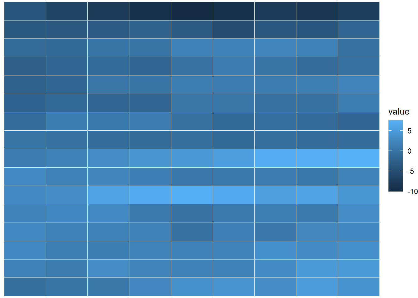
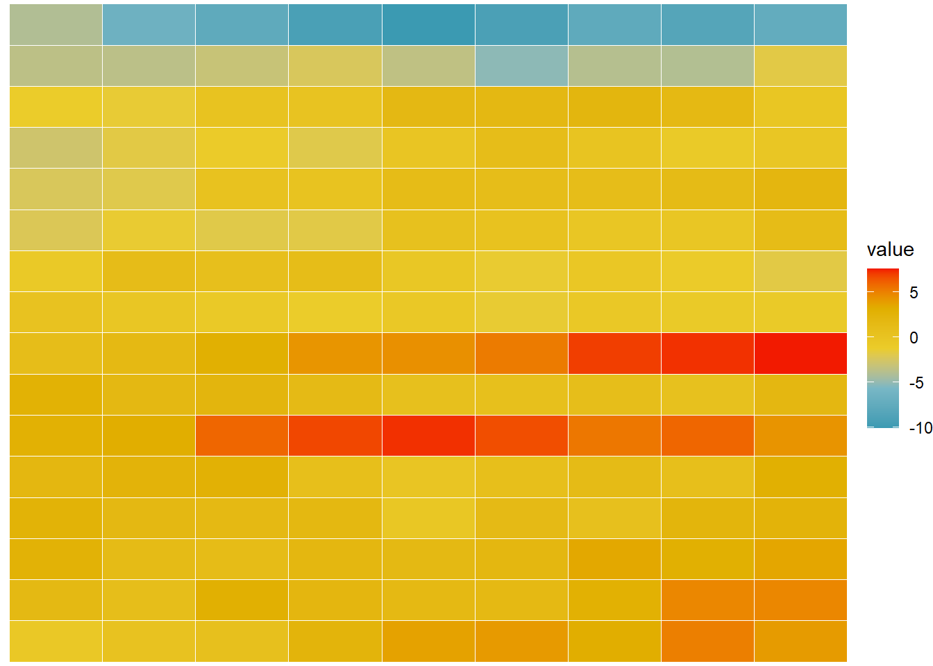
}The Figure 3 (b) demonstrates the use of this scale_fill_wesanderson() function using a dataset heatmap from {wesanderson} package itself. (Ram and Wickham 2023).
Code
q4_1 <- wesanderson::heatmap |>
  ggplot(aes(Var1, Var2, fill = value)) +
  geom_tile(color = "white") +
  theme_void()

q4_1
q4_1 +
  scale_fill_wesanderson(
    palette = "Zissou1",
    type = "continuous"
    )
18.3.4 Exercises
Question 1
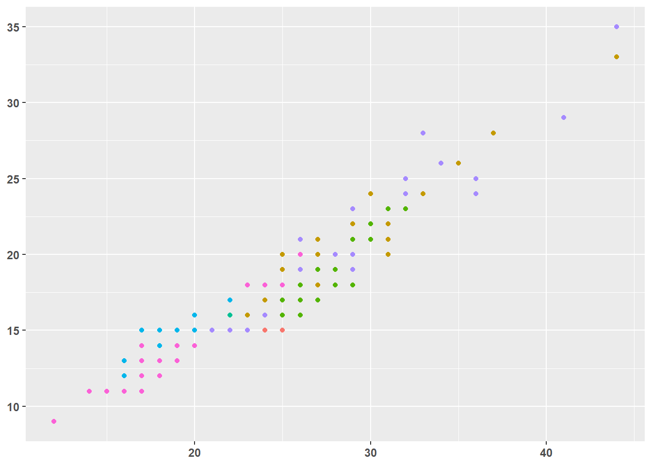
To make the best use of space, many examples in this book hide the axes labels and legend. we’ve just copied-and-pasted the same code into multiple places, but it would make more sense to create a reusable function. What would that function look like?
We may use a custom function, theme_bookprint() as follows: –
theme_bookprint <- function(...){
  theme(
    axis.title = element_blank(),
    legend.position = "none",
    ...
  )}
The following Figure 4 (b) demonstrates the use of this custom function.
Code
# The raw plot
g1 <- ggplot(mpg, aes(hwy, cty, col = class)) + geom_point()

theme_bookprint <- function(...){
  theme(
    axis.title = element_blank(),
    legend.position = "none",
    ...
  )
}

g1

g1 +
  theme_bookprint(axis.text = element_text(face = "bold"))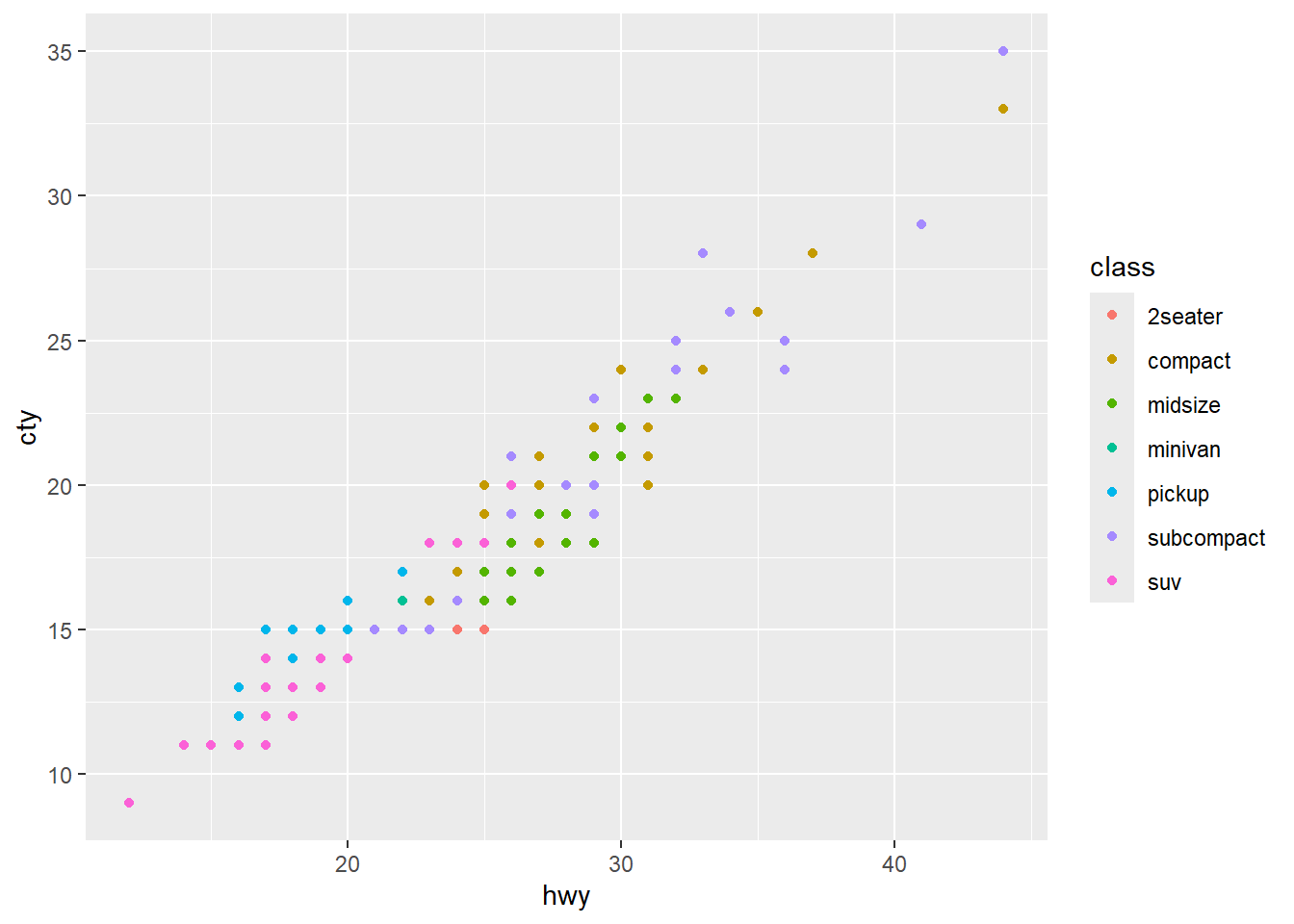
Question 2
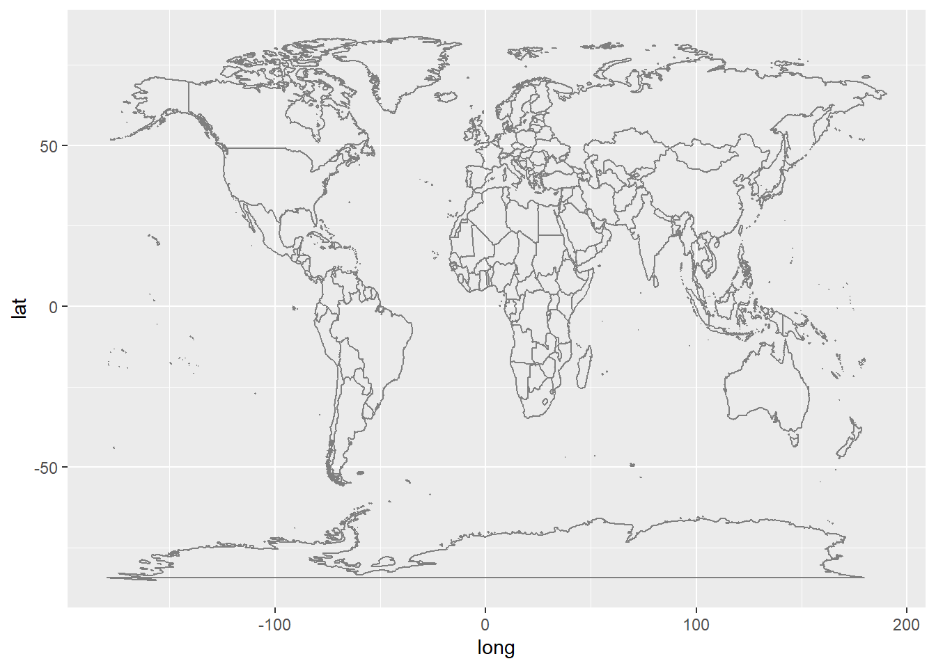
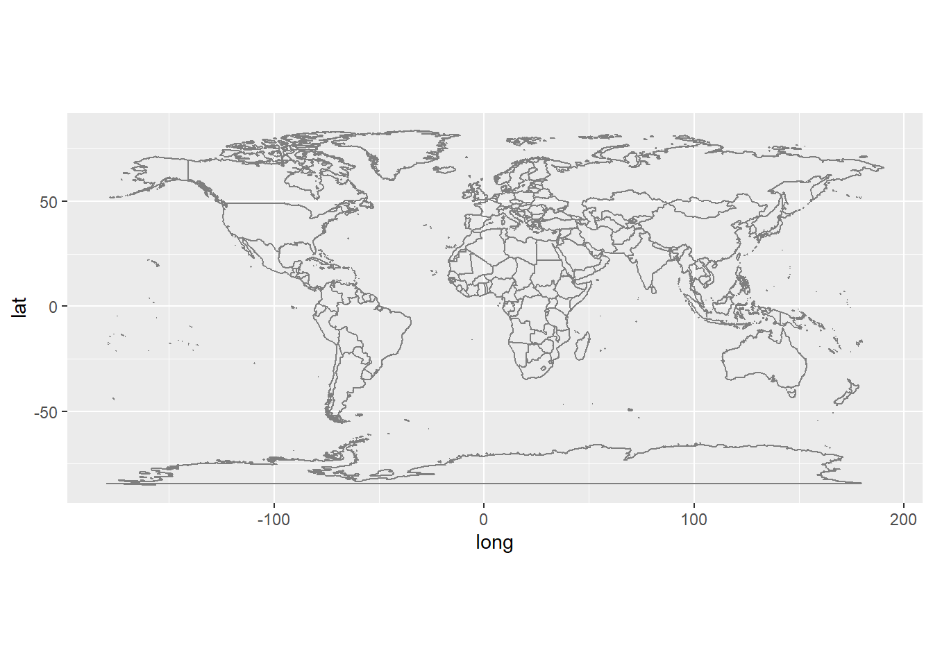
Extend the borders() function to also add coord_quickmap() to the plot.
The new custom_borders() extending upon the original borders() function will looks like this:
custom_borders <- function(...) {
  list(
    borders(...),
    coord_quickmap()
  )
}
The Figure 5 (b) shows application of the custom_borders() to the world map
Code
Question 3
Look through your own code. What combinations of geoms or scales do you use all the time? How could you extract the pattern into a reusable function?
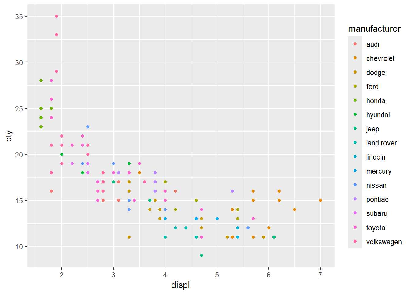
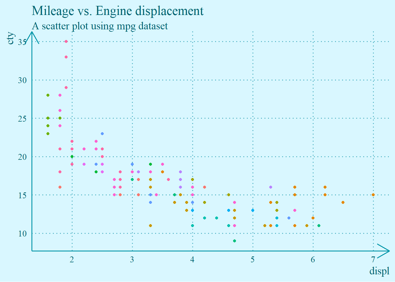
In my plots, I often remove the legend, put axes-labels at the end on axes, and remove margins around the plot titles, subtitles and axes texts. I even remove axis ticks at many times. Further, I like to choose a bacground colour, and change all other text and line colours to its darker versions accordingly. Now, the Figure 6 (b) demonstrates an example of this.
Code
g2 <- mpg |>
  ggplot(aes(y = cty, x = displ, colour = manufacturer)) +
  geom_point()

custom_plot <- function(title = "", subtitle = "",
                        background = "grey95", ...){
  list(
    labs(title = title, subtitle = subtitle),
    theme_minimal(base_size = 14, base_family = "serif"),
    theme(
      legend.position = "none",
      axis.line = element_line(
        arrow = arrow(),
        colour = colorspace::darken(background, 0.4)
      ),
      axis.text = element_text(
        colour = colorspace::darken(background, 0.6)
      ),
      axis.title = element_text(
        colour = colorspace::darken(background, 0.6),
        hjust = 1
      ),
      panel.grid.major = element_line(
        linetype = 3,
        colour = colorspace::darken(background, 0.3)
      ),
      panel.grid.minor = element_blank(),
      axis.ticks = element_blank(),
      plot.title = element_text(
        margin = margin(0,0,5,0),
        colour = colorspace::darken(background, 0.6)
      ),
      plot.subtitle = element_text(
        margin = margin(0,0,0,0),
        colour = colorspace::darken(background, 0.6)
      ),
      plot.background = element_rect(fill = background, colour = NA),
      ...
    )
  )
}


g2

g2 + custom_plot(
  "Mileage vs. Engine displacement",
  "A scatter plot using mpg dataset",
  background = "#d9f7ff")