Chapter 17

Themes

Author

Aditya Dahiya

Published

March 29, 2024

This chapter has some exercises. I also demonstrate some other features using sample data sets.

Code

library(tidyverse)
library(scales)
library(ggthemes)
library(gt)

17.1 Introduction

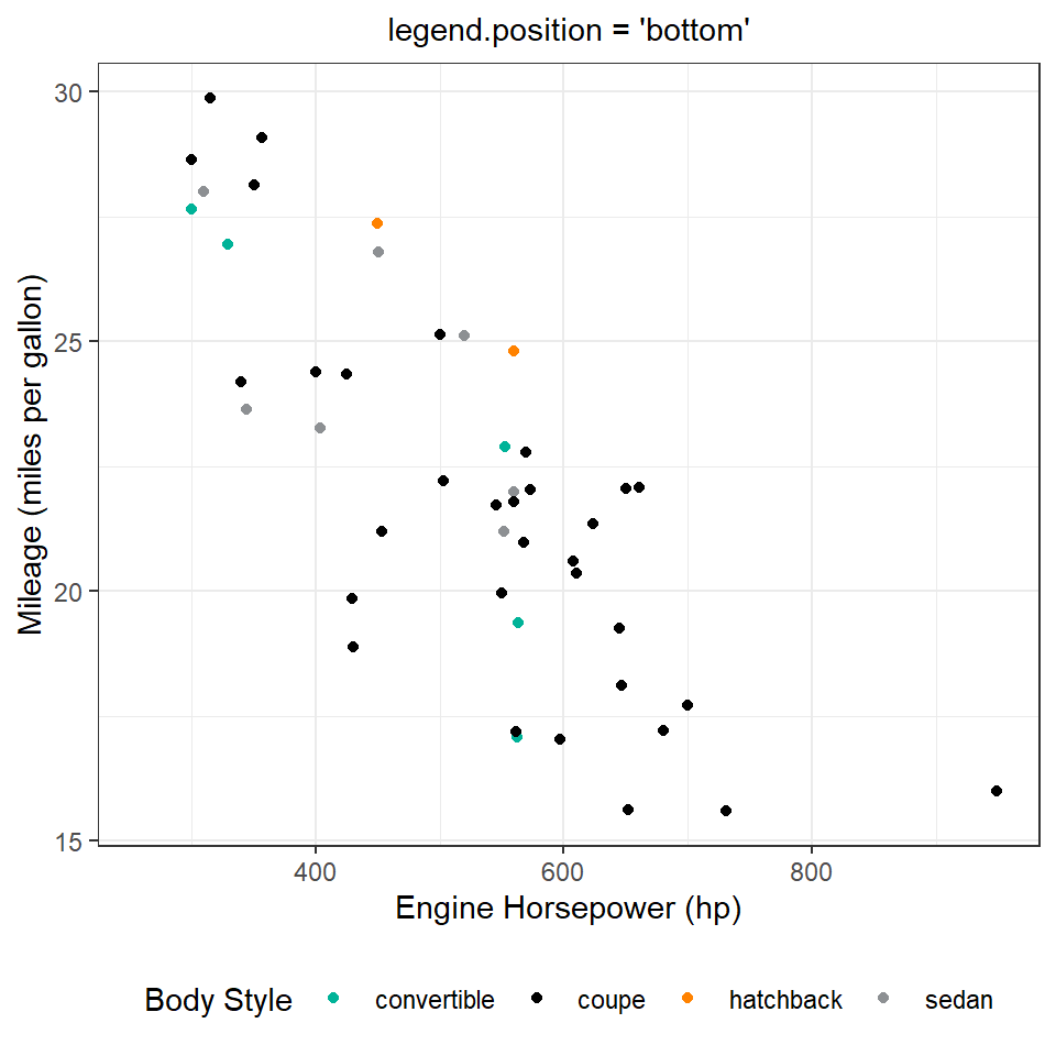
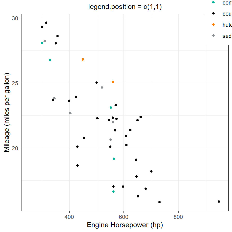
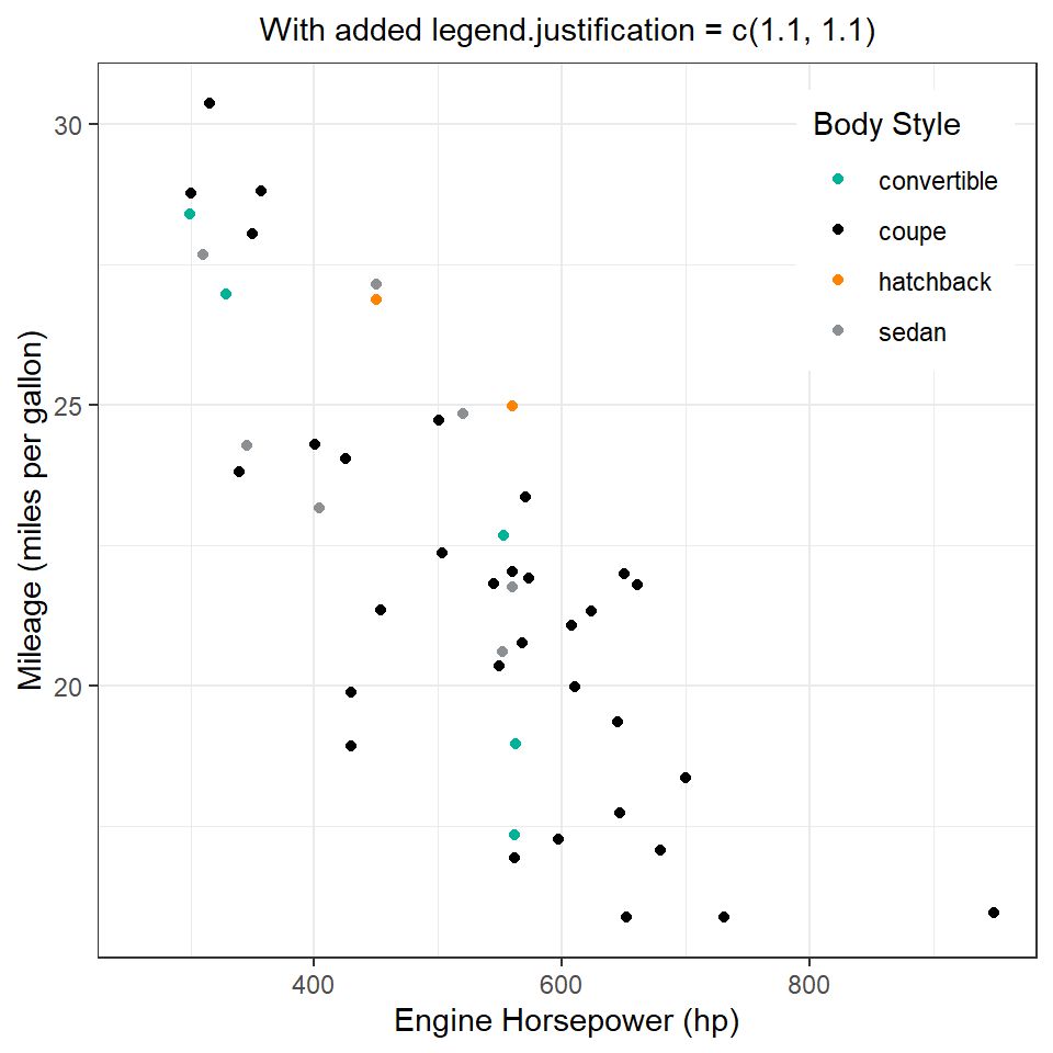
A demonstration on the use of legend.position = "" and legend.justification = "" with the function theme() function of the ggplot2 is shown in Figure 1 . As we can see in Figure 1 (d), using both arguments together produces the best result.

Code

g1 <- gt::gtcars |> 
  ggplot(aes(hp, mpg_h, colour = bdy_style)) +
  geom_jitter() +
  labs(
    x = "Engine Horsepower (hp)",
    y = "Mileage (miles per gallon)",
    colour = "Body Style"
  ) +
  paletteer::scale_colour_paletteer_d("nbapalettes::clippers_original") +
  theme_bw() +
  theme(plot.subtitle = element_text(hjust = 0.5))

g1 + labs(subtitle = "Base Plot")

g1 + theme(legend.position = "bottom") + labs(subtitle = "legend.position = 'bottom'")

g1 +
  theme(legend.position = c(1,1)) + 
  labs(subtitle = "legend.position = c(1,1)")

g1 + 
  theme(legend.position = c(1,1),
        legend.justification = c(1.1, 1.1)) +
  labs(subtitle = "With added legend.justification = c(1.1, 1.1)")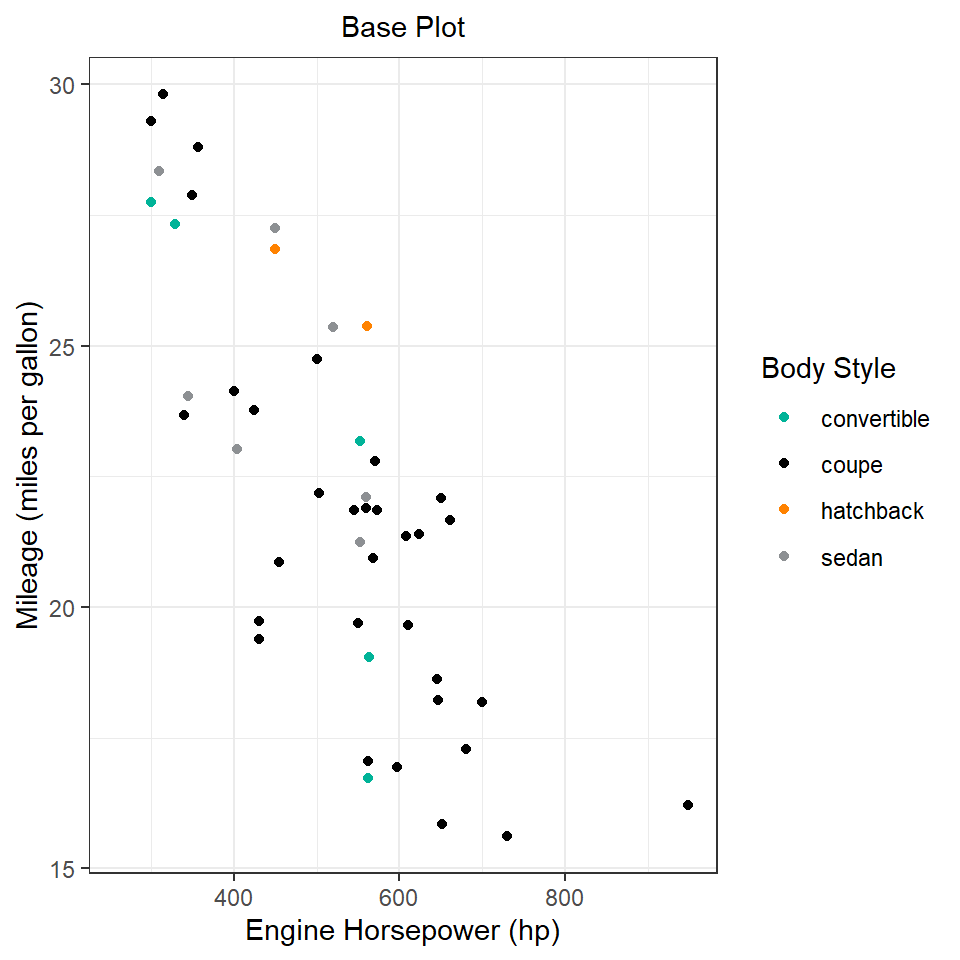

17.2 Complete themes

A very good argument to use with theme_*() family of functions is the base_size = argument to fix a base size for all text used in the plot, and base_family = to set the font for the entire plot.

17.2.1 Exercises

Question 1

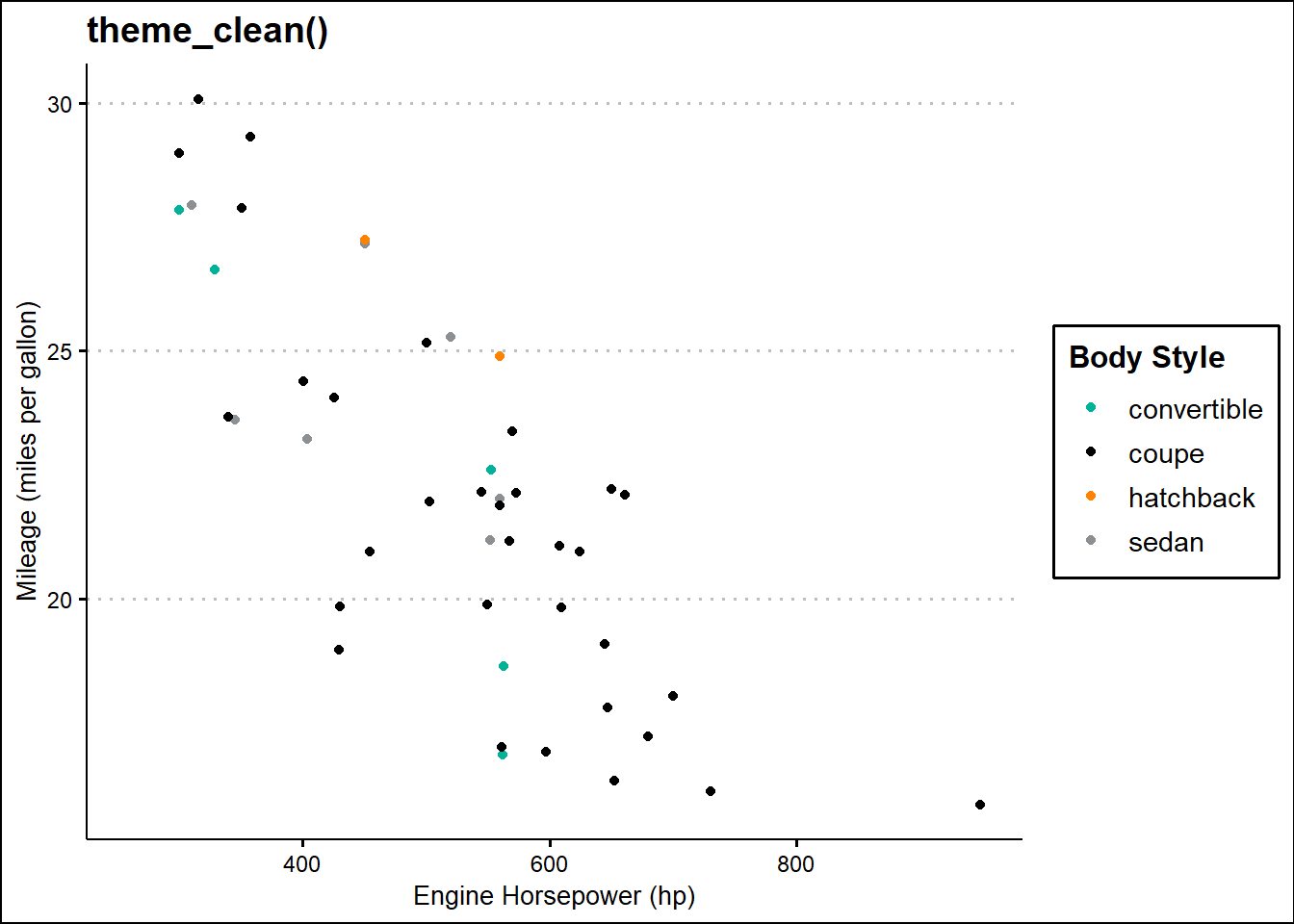
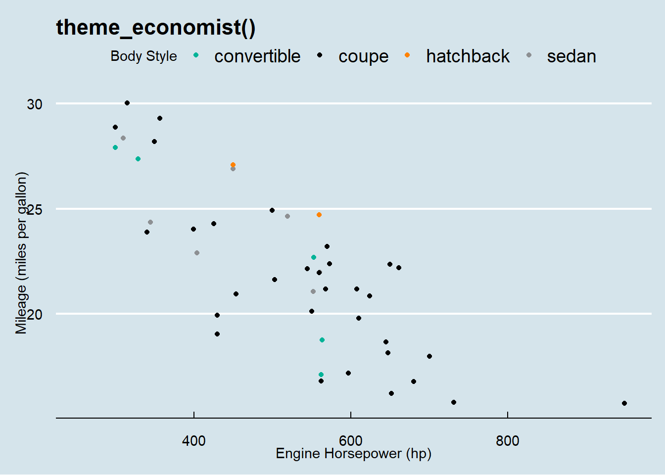
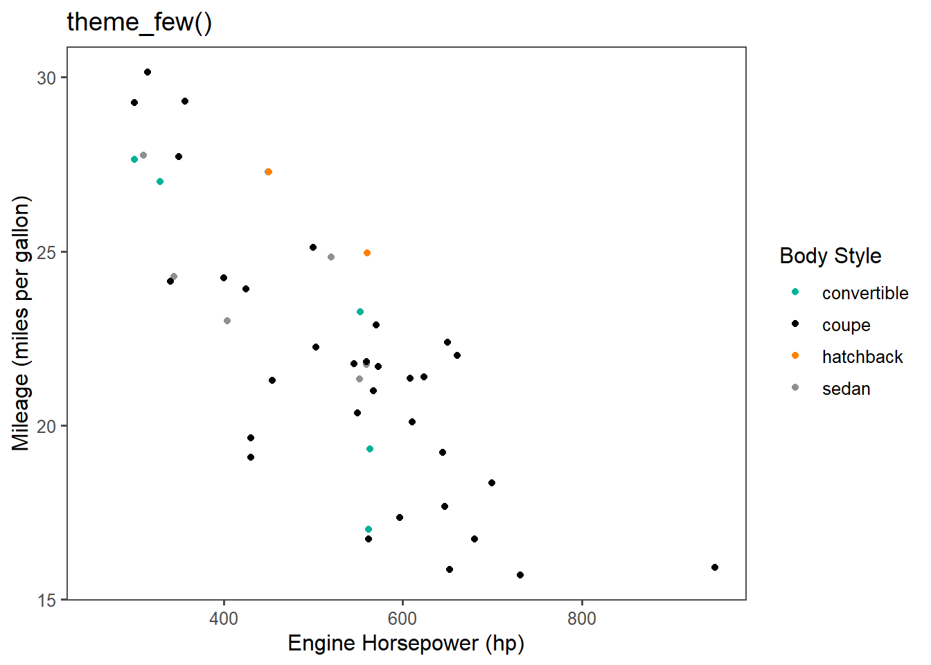
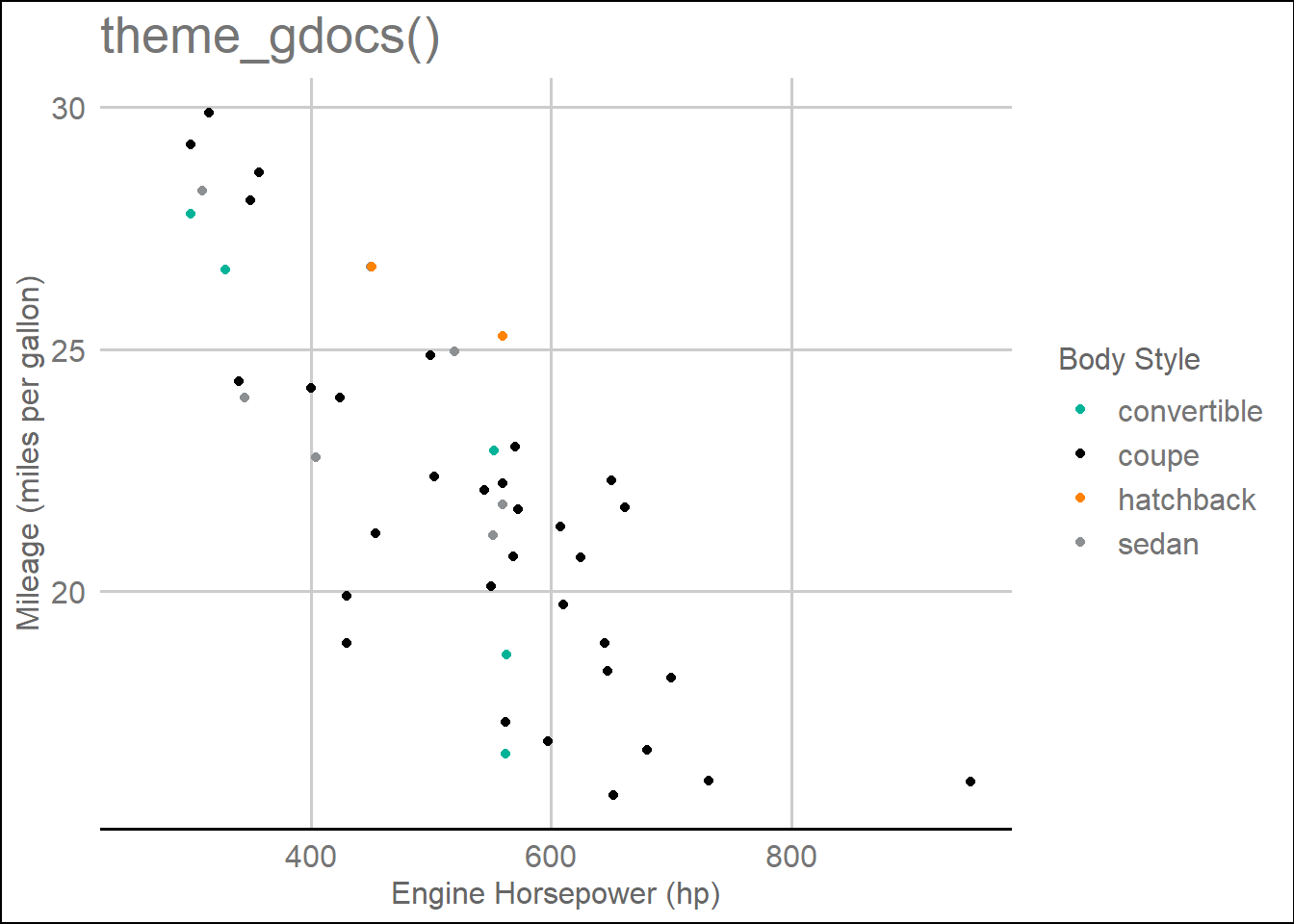
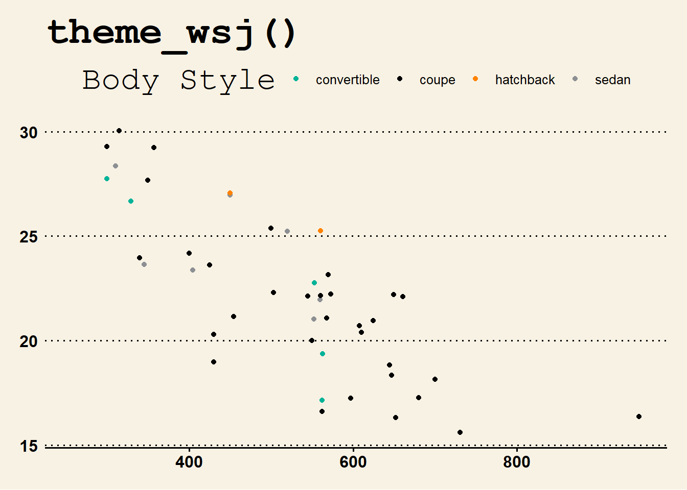
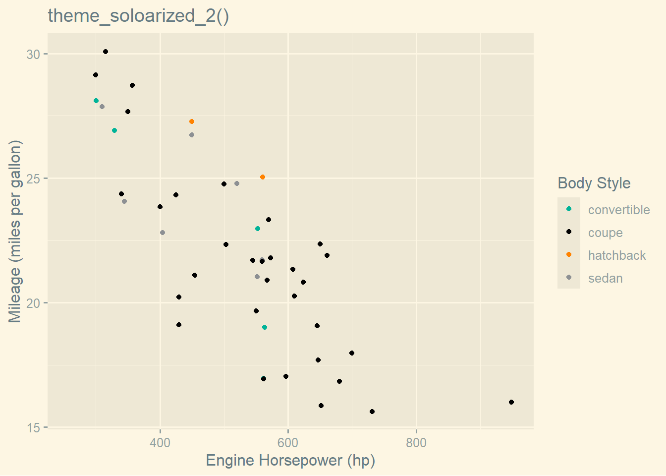
Try out all the themes in `ggthemes`. Which do you like the best?

The various themes of ggthemes are shown in Figure 2. The best one seems to be theme_clean() as it allows easy customization.

Code

g2 <- g1 + theme(legend.position = "bottom")

g2 + ggthemes::theme_calc() + ggtitle("theme_calc()")

g2 + ggthemes::theme_clean() + ggtitle("theme_clean()")

g2 + ggthemes::theme_economist() + ggtitle("theme_economist()")

g2 + ggthemes::theme_excel_new() + ggtitle("theme_excel_new()")

g2 + ggthemes::theme_few() + ggtitle("theme_few()")

g2 + ggthemes::theme_gdocs() + ggtitle("theme_gdocs()")

g2 + ggthemes::theme_wsj() + ggtitle("theme_wsj()")

g2 + ggthemes::theme_solarized_2() + ggtitle("theme_soloarized_2()")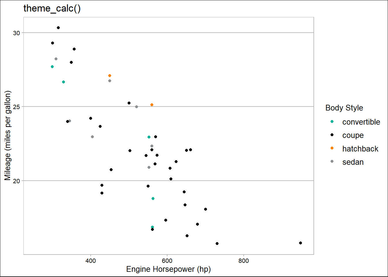

Question 2

What aspects of the default theme do you like? What don’t you like?
What would you change?

In ggplot2, the default theme (theme_gray()) has several aspects that align well with Tufte’s principles and are conducive to clear and effective data visualization:

Minimalist Design: The default theme employs a clean and minimalist design, which is in line with Tufte’s principle of maximizing data-ink ratio. This means that unnecessary elements are minimized, allowing the data to stand out more prominently.
Neutral Background: The light gray background in the default theme provides a neutral canvas for the data to be presented on. This is generally preferable for readability, especially when using a white background, as it reduces contrast and minimizes visual distractions.
Simple Grid Lines: The faint grid lines in the default theme help guide the viewer’s eye across the plot without overpowering the data.

However, there are a few aspects of the default theme that could be improved to better align with Tufte’s principles, which I generally follow,: —

Thinner Axes and Tick Marks: Tufte suggests using thinner axes and tick marks to further reduce visual clutter and draw attention to the data. The default theme could benefit from thinner lines for both axes and tick marks.
Increased Font Size for Labels and Titles: While the default font size is generally adequate, increasing the font size slightly for axis labels, titles, and annotations can enhance readability, especially when viewing plots from a distance or on smaller screens.
Adjustment of Plot Margins: Tufte emphasizes the importance of maximizing the data-ink ratio by minimizing non-data ink, including unnecessary margins. Adjusting the default plot margins to be more compact could help achieve this goal and allow for more space dedicated to the presentation of data.

Overall, while the default theme in ggplot2 aligns well with Tufte’s principles in many aspects, there are opportunities for further refinement to enhance clarity, simplicity, and effectiveness in data visualization. These suggested changes aim to optimize the balance between aesthetic appeal and functional clarity in accordance with Tufte’s principles.

Question 3

Look at the plots in your favourite scientific journal. What theme do they most resemble? What are the main differences?

In many scientific journals, especially those focused on data visualization and analysis, the plots often resemble themes that prioritize clarity, simplicity, and effective communication of information. One common theme that many plots in scientific journals resemble is the “classic” theme in ggplot2, which emphasizes clean lines, minimal distractions, and a focus on the data itself.

The example image for a graph / plot from the journal Nature is given below:

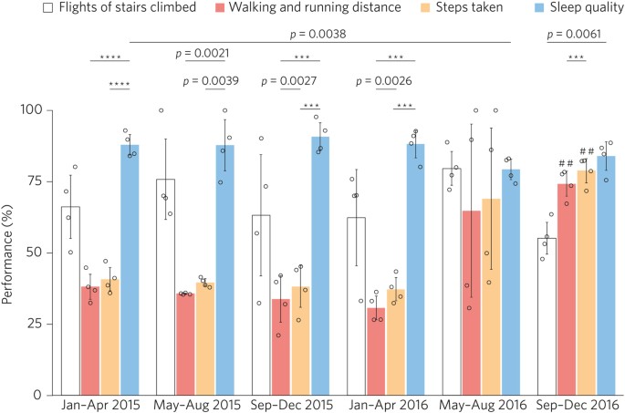
Credits: https://media.springernature.com/m685/springer-static/image/art%3A10.1038%2Fs41551-017-0079/MediaObjects/41551_2017_Article_BFs415510170079_Fig1_HTML.jpg

The main differences between the plots in scientific journals and the “classic” ggplot2 theme lie in the specific customizations and adjustments made to suit the needs of the particular journal’s style and the preferences of its audience. Here are some of the main differences that may be observed:

Color Palette: Scientific journals often have specific guidelines for color usage, particularly for distinguishing between different groups or conditions in the data. While the “classic” ggplot2 theme uses a simple default color palette, plots in scientific journals may employ custom color schemes that adhere to the journal’s style guidelines.
Font Choices: Journals typically have standardized fonts for text, including axis labels, titles, and annotations. While ggplot2 allows for customization of fonts, plots in scientific journals may use fonts that match the journal’s style guide, which may differ from the default fonts in ggplot2.
Axis and Tick Mark Styles: The style and thickness of axes and tick marks may be adjusted in scientific journal plots to match the journal’s aesthetic preferences or to enhance readability. This could include changes such as thinner lines, different line styles, or adjustments to the length and spacing of tick marks.
Annotation and Labeling: Scientific journal plots often include detailed annotations, such as significance indicators, error bars, or additional text descriptions. These annotations may be placed strategically to ensure clarity and precision in conveying the results of the analysis.
Plot Aspect Ratio and Size: The aspect ratio and overall size of plots in scientific journals may be adjusted to fit within the journal’s page layout and to optimize presentation on both digital and print platforms. This could involve resizing plots to ensure they are legible and visually appealing at different scales.

Overall, while plots in scientific journals share similarities with the “classic” ggplot2 theme in their emphasis on clarity and simplicity, they often incorporate customization to align with the journal’s style guidelines and the preferences of its audience. These customization aim to enhance the effectiveness of the visual communication of data within the context of the specific publication.

17.3 Modifying theme components

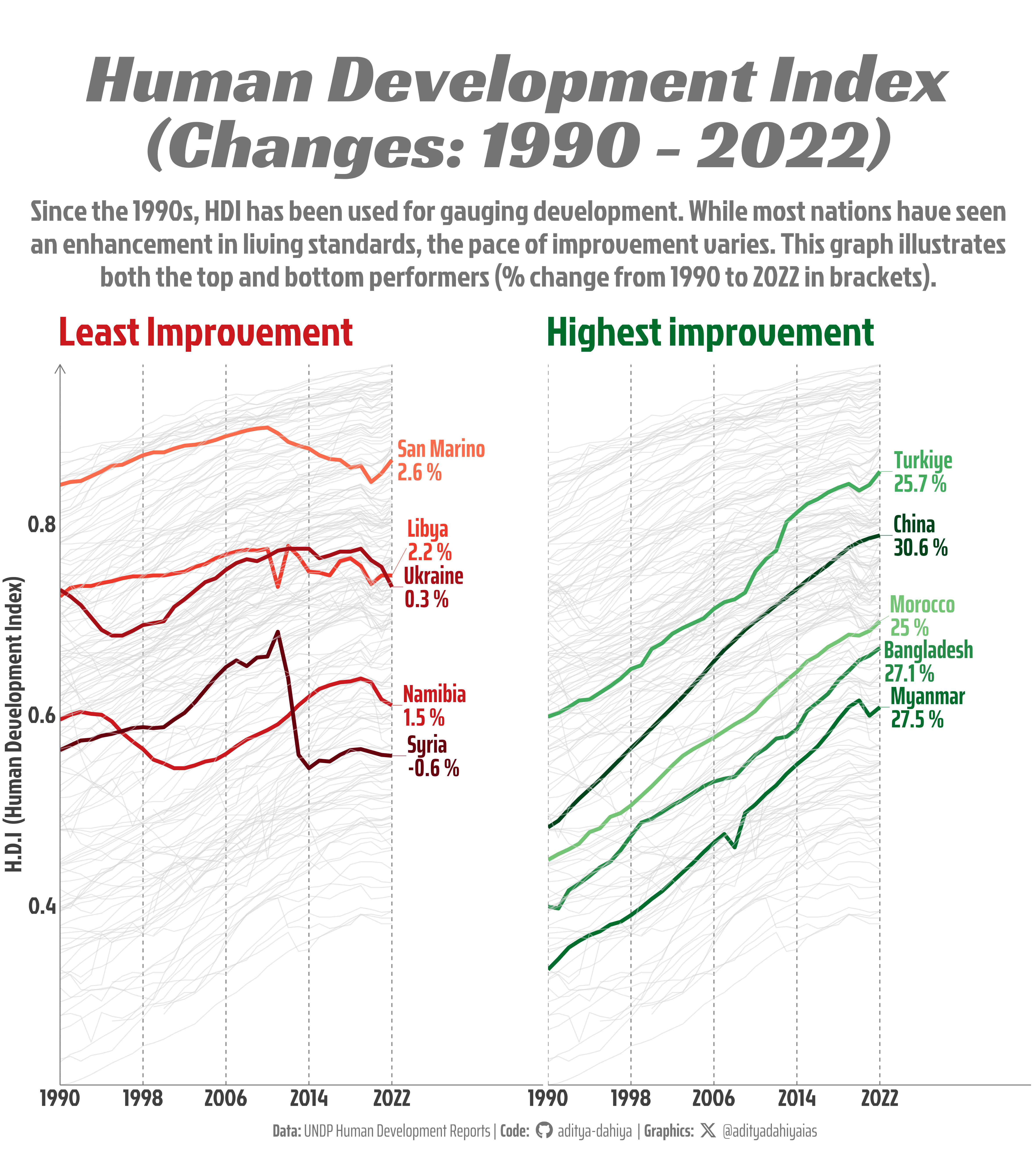
The example in Figure 3 shows heavy customization of the theme elements. The code is also given below.

Code

# =============================================================================#
# About the Dataset-------------------------------------------------------------
# =============================================================================#

# Source URL: https://hdr.undp.org/data-center/documentation-and-downloads
# Credits: UNDP Human Development Reports
# Human development, quantified. One of the most widely recognized measures, 
# the United Nations' Human Development Index amalgamates data on life 
# expectancy, per capita income, and educational attainment into a singular 
# value for each country-year. The UN offers downloadable files and an API 
# encompassing all yearly HDI rankings and sub-indicators spanning from 1990 to
# 2022. These resources also encompass information from correlated indices like 
# the Inequality-adjusted Human Development Index, Gender Development Index, and 
# Gender Inequality Index.

# =============================================================================#
# Findings ---------------------------------------------------------------------
# =============================================================================#

# The best performing countries, in terms of HDI improvement between 1990 and 
# 2022 are: China, Myanmar, Bangladesh, Turkiye, and, Morocco
# The wrost performing countries, in terms of HDI reduction / least increase
# between 1990 and 2022 are: Syria, Ukraine, Namibia, Libya, and, San Marino

# =============================================================================#
# Library Load-in---------------------------------------------------------------
# =============================================================================#

# Data Wrangling Tools
library(tidyverse)
library(janitor)
library(here)
library(sf)

# Final plot (ggplot2) tools
library(scales)
library(fontawesome)
library(ggtext)
library(showtext)
library(colorspace)


# =============================================================================#
# Data Load-in, EDA & Data Wrangling--------------------------------------------
# =============================================================================#

# Read in the UNDP data
url <- "https://hdr.undp.org/sites/default/files/2023-24_HDR/HDR23-24_Composite_indices_complete_time_series.csv"

hdi <- read_csv(url)

# Number of countries to highlight in each
nos <- 5

# A wide format and housekeeping to filter out relevant variables, and also
# change names of some countries to easily recognizable names
dfwide <- hdi |> 
  select(iso3, 
         country, 
         region, 
         (contains("hdi_") & !(contains("_m_")) & !(contains("_f_")) & !(contains("ihdi")) & !(contains("phdi")) & !(contains("rank"))
          )
         ) |> 
  filter(!(country %in% c("East Asia and the Pacific"))) |> 
  mutate(country = if_else(country == "T\xfcrkiye", "Turkiye", country),
         country = if_else(country == "Syrian Arab Republic", "Syria", country))

# Long (tidy) format of the data (needed for plotting facets in ggplot2)
df1 <- dfwide |> 
  pivot_longer(
    cols = contains("hdi"),
    names_to = "year",
    values_to = "value"
  ) |> 
  mutate(year = parse_number(year))

# Improvement amongst countries
df_imp <- dfwide |> 
  mutate(improvement = hdi_2022 - hdi_1990) |> 
  select(country, improvement)

# Worst off countries
least_imp <- df_imp |> 
  slice_min(order_by = improvement, n = nos) |> 
  pull(country)

# Best improvement countries
most_imp <- df_imp |> 
  slice_max(order_by = improvement, n = nos) |> 
  pull(country)

least_imp
most_imp
# A tibble for actual percentage change in HDI - to show in graph
changes <- bind_rows(
  df_imp |> 
    slice_min(order_by = improvement, n = nos),
  df_imp |> 
    slice_max(order_by = improvement, n = nos)
) |> 
  mutate(
    improvement = round(100 * improvement, 1)
  )

# Tibble to actually use in plotting
plotdf <- df1 |> 
  mutate(
    most_improved = if_else(country %in% most_imp, country, NA),
    least_improved= if_else(country %in% least_imp, country, NA)
  ) |> 
  pivot_longer(
    cols = c(most_improved, least_improved),
    names_to = "facet_var",
    values_to = "colour_var"
  ) |> 
  mutate(colour_var = fct(colour_var, levels = c(least_imp, most_imp))) |> 
  left_join(changes)
# =============================================================================#
# Options & Visualization Parameters--------------------------------------------
# =============================================================================#

# Load fonts
# Font for titles
font_add_google("Racing Sans One",
  family = "title_font"
) 

# Font for the caption
font_add_google("Saira Extra Condensed",
  family = "caption_font"
) 

# Font for plot text
font_add_google("Jockey One",
  family = "body_font"
) 

showtext_auto()

# Define colours
reds <- paletteer::paletteer_d("RColorBrewer::Reds", direction = -1)[1:nos]
greens <- paletteer::paletteer_d("RColorBrewer::Greens", direction = -1)[1:nos]
mypal <- c(reds, greens)


bg_col <- "#ffffff"   # Background Colour
text_col <- "#404040" # Colour for the text
text_hil <- '#757575' # Colour for highlighted text

# Define Text Size
ts <- unit(20, units = "cm") # Text Size

# Caption stuff
sysfonts::font_add(
  family = "Font Awesome 6 Brands",
  regular = here::here("docs", "Font Awesome 6 Brands-Regular-400.otf")
)
github <- "&#xf09b"
github_username <- "aditya-dahiya"
xtwitter <- "&#xe61b"
xtwitter_username <- "@adityadahiyaias"
social_caption_1 <- glue::glue("<span style='font-family:\"Font Awesome 6 Brands\";'>{github};</span> <span style='color: {text_hil}'>{github_username}  </span>")
social_caption_2 <- glue::glue("<span style='font-family:\"Font Awesome 6 Brands\";'>{xtwitter};</span> <span style='color: {text_hil}'>{xtwitter_username}</span>")


# Add text to plot--------------------------------------------------------------
plot_title <- "Human Development Index\n(Changes: 1990 - 2022)"
plot_caption <- paste0("**Data:** UNDP Human Development Reports", " | ", " **Code:** ", social_caption_1, " | ", " **Graphics:** ", social_caption_2)
subtitle_text <- "Since the 1990s, HDI has been used for gauging development. While most nations have seen an enhancement in living standards, the pace of improvement varies. This graph illustrates both the top and bottom performers (% change from 1990 to 2022 in brackets)."
plot_subtitle <- str_wrap(subtitle_text, 90)

# ==============================================================================#
# Data Visualization------------------------------------------------------------
# ==============================================================================#

strip_text <- c(
  "<b style='color:#CB181DFF'>Least Improvement</b>", 
  "<b style='color:#006D2CFF'>Highest improvement</b>"
  )
names(strip_text) <- c("least_improved", "most_improved")

g <- plotdf |> 
  ggplot(
    aes(
      x = year,
      y = value,
      group = country,
      color = colour_var,
      alpha = is.na(colour_var),
      linewidth = is.na(colour_var)
    )
  ) +
  geom_line() +
  ggrepel::geom_text_repel(
    data = (plotdf |> filter(year == 2022)),
    mapping = aes(
      label = if_else(
        !is.na(colour_var),
        paste0(colour_var, "\n", improvement, " %"),
        NA
      )
    ),
    force        = 10,
    nudge_x      = 2.5,
    direction    = "y",
    hjust        = 0,
    segment.size = 0.2,
    size = 30,
    lineheight = 0.25,
    family = "caption_font",
    fontface = "bold",
    box.padding = 0
  ) +
  facet_wrap(
    ~ facet_var,
    labeller = labeller(facet_var = strip_text)
  ) +
  scale_x_continuous(
    expand = expansion(c(0, 0.35)),
    breaks = seq(1990, 2022, 8)
  ) +
  scale_y_continuous(
    expand = expansion(0)
  ) +
  scale_alpha_discrete(range = c(1, 0.5)) +
  scale_linewidth_discrete(range = c(2, 0.5)) +
  scale_colour_manual(
    values = mypal,
    na.value = "lightgrey"
  ) +
  labs(
    title = plot_title,
    subtitle = plot_subtitle,
    caption = plot_caption,
    x = NULL,
    y = "H.D.I  (Human Development Index)"
  ) +
  theme_minimal(
     base_family = "body_font"
  ) +
  theme(
    legend.position = "none",
    panel.grid.minor = element_blank(),
    panel.grid.major.y = element_line(
      linewidth = 0.5,
      colour = "transparent"
    ),
    panel.grid.major.x = element_line(
      linewidth = 0.5,
      linetype = 2,
      colour = text_hil
    ),
    axis.line.x = element_line(
      colour = text_hil,
      linewidth = 0.5
    ),
    axis.line.y = element_line(
      colour = text_hil,
      linewidth = 0.5,
      arrow = arrow(length = unit(0.4, "cm"))
    ),
    plot.title.position = "plot",
    plot.title = element_text(
      colour = text_hil,
      hjust = 0.5,
      family = "title_font",
      size = 12 * ts,
      margin = margin(2,0,0.25,0, "cm"),
      lineheight = 0.25
    ),
    plot.subtitle = element_text(
      hjust = 0.5,
      lineheight = 0.3,
      colour = text_hil,
      size = 5 * ts,
      margin = margin(0,0,1,0, "cm")
    ),
    axis.text = element_text(
      colour = text_col,
      hjust = 0.5,
      margin = margin(0,0,0,0),
      size = 4 * ts
    ),
    axis.title = element_text(
      colour = text_col,
      hjust = 0.5,
      margin = margin(0,0,0,0),
      size = 4 * ts
    ),
    plot.caption = element_textbox(
      family = "caption_font",
      colour = text_hil,
      size = 3 * ts,
      hjust = 0.5,
      margin = margin(0.5,0,0.8,0, "cm")
    ),
    strip.text = element_markdown(
      family = "body_font",
      size = 7 * ts,
      margin = margin(0,0,0.5,0, "cm")
    )
  )


# =============================================================================#
# Image Saving-----------------------------------------------------------------
# =============================================================================#

ggsave(
  filename = here::here("docs", "dip_hdi.png"),
  plot = g,
  width = 40,
  height = 45,
  units = "cm",
  bg = bg_col
)

Figure 3: Heavily customized theme elements using element_text(), element_line() and element_rect()

17.4 Theme elements

17.4.6 Exercises

Question 1

Create the ugliest plot possible! (Contributed by Andrew D. Steen, University of Tennessee - Knoxville)

The example plot, one of the ugliest one can think of, is shown in Figure 4

Code

# Load necessary libraries
library(ggplot2)
library(dplyr)

# Load mtcars dataset
data(mtcars)

# Create an intentionally ugly plot
ggplot(mtcars, aes(x = wt, y = mpg)) +
  geom_point(color = "red", size = 5, shape = 18) +
  geom_smooth(method = "lm", color = "blue", fill = "green", alpha = 0.3, size = 2) +
  scale_x_continuous("Car Weight (1000 lbs)", breaks = seq(0, 6, by = 1), labels = c("0", "1", "2", "3", "4", "5", "6")) +
  scale_y_continuous("Miles/(US) gallon", breaks = seq(10, 35, by = 5), labels = c("10", "15", "20", "25", "30", "35")) +
  theme_minimal(base_family = "Comic Sans MS", base_size = 20) +
  theme(panel.background = element_rect(fill = "black"),
        panel.grid.major = element_line(color = "purple", size = 1.5),
        panel.grid.minor = element_line(color = "orange", size = 0.5),
        axis.line = element_line(color = "yellow", size = 2),
        axis.title = element_text(color = "red", size = 30, face = "bold"),
        axis.text = element_text(color = "blue", size = 25, angle = 45, hjust = 1, vjust = 1),
        axis.ticks = element_line(color = "green", size = 1.5),
        plot.title = element_text(color = "brown", size = 40, face = "italic", hjust = 0.5),
        plot.subtitle = element_text(color = "magenta", size = 30, face = "bold", hjust = 0.5),
        plot.caption = element_text(color = "cyan", size = 20, face = "italic", hjust = 1),
        legend.title = element_text(color = "orange", size = 20, face = "bold"),
        legend.text = element_text(color = "purple", size = 15),
        legend.background = element_rect(fill = "yellow", color = "green", size = 1.5),
        legend.key = element_rect(fill = "blue", color = "red", size = 2),
        legend.position = "bottom",
        legend.direction = "vertical",
        legend.box = "vertical",
        legend.key.size = unit(2, "cm"),
        plot.background = element_rect(fill = "grey"))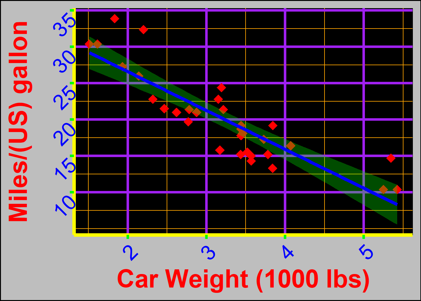

Figure 4: The ugliest possible plot! Everything is too bright and out of order!

Question 2

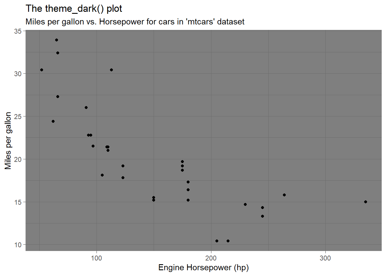
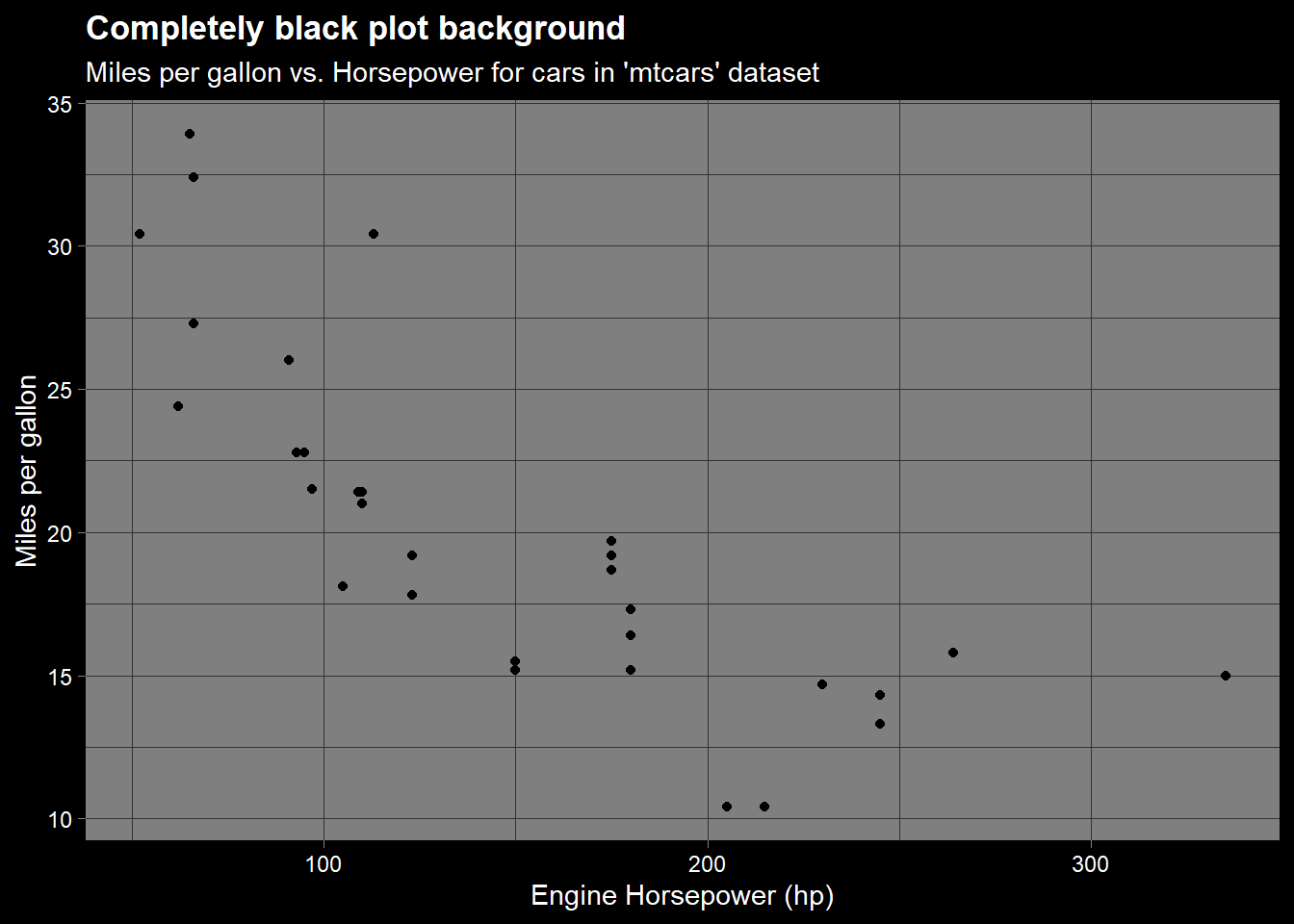
theme_dark() makes the inside of the plot dark, but not the outside. Change the plot background to black, and then update the text settings so you can still read the labels.

Code

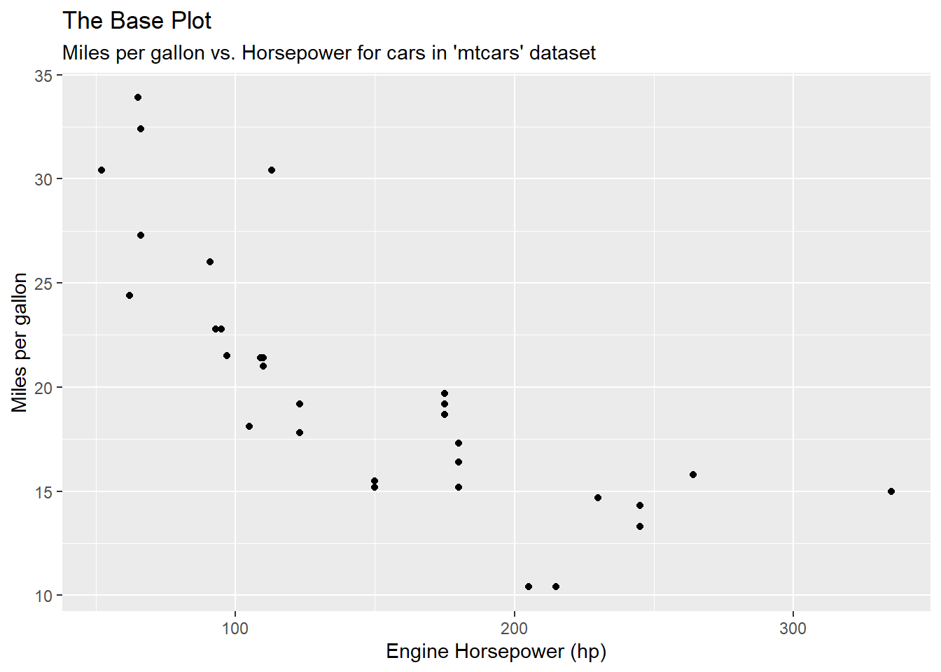
g1 <- ggplot(mtcars, aes(hp, mpg)) +
  geom_point() +
  labs(
    subtitle = "Miles per gallon vs. Horsepower for cars in 'mtcars' dataset",
    x = "Engine Horsepower (hp)",
    y = "Miles per gallon"
    )

g1 + ggtitle("The Base Plot")

g1 + ggtitle("The theme_dark() plot") + theme_dark()

g1 + ggtitle("Completely black plot background") +
  theme_dark() +
  theme(
    plot.background = element_rect(fill = "black", colour = "black"),
    plot.title = element_text(colour = "white", face = "bold"),
    plot.subtitle = element_text(colour = "white"),
    axis.title = element_text(colour = "white"),
    axis.text = element_text(colour = "white"),
    axis.ticks = element_line(colour = "grey50"),
    panel.grid = element_line(colour = "grey20")
  )

Question 3

Make an elegant theme that uses “linen” as the background colour and a serif font for the text.

Code

library(showtext)
font_add_google("Marcellus", "serif_font")
showtext_auto()
g1 +
  ggtitle("A nice serif font and linen background for the plot") +
  theme_clean(base_family = "serif_font", base_size = 18) +
  theme(
    plot.background = element_rect(fill = "linen"),
    plot.title = element_text(face = "bold", size = 27)
  )

Figure 6: Using linen as plot background and a serif font

Question 4

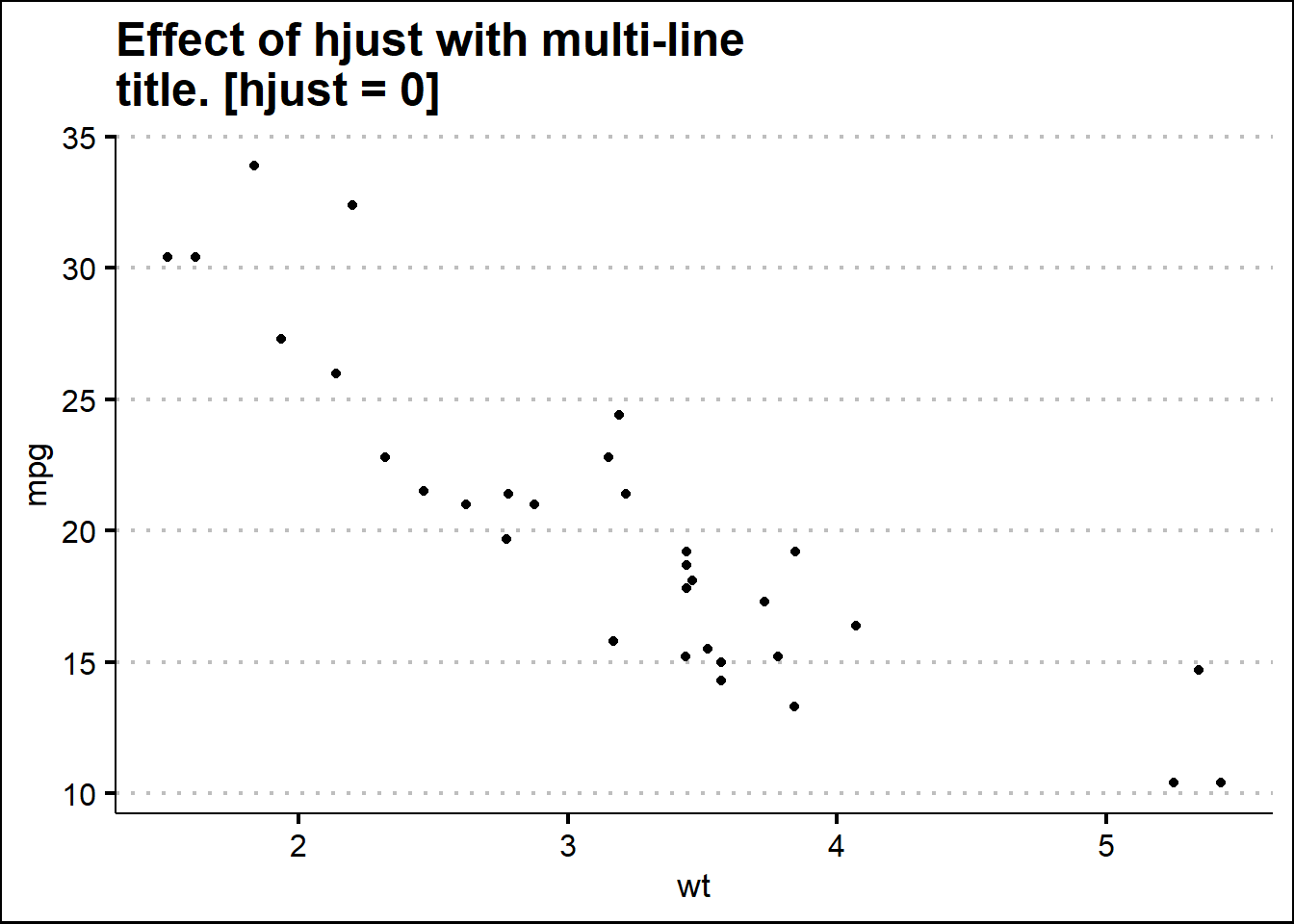
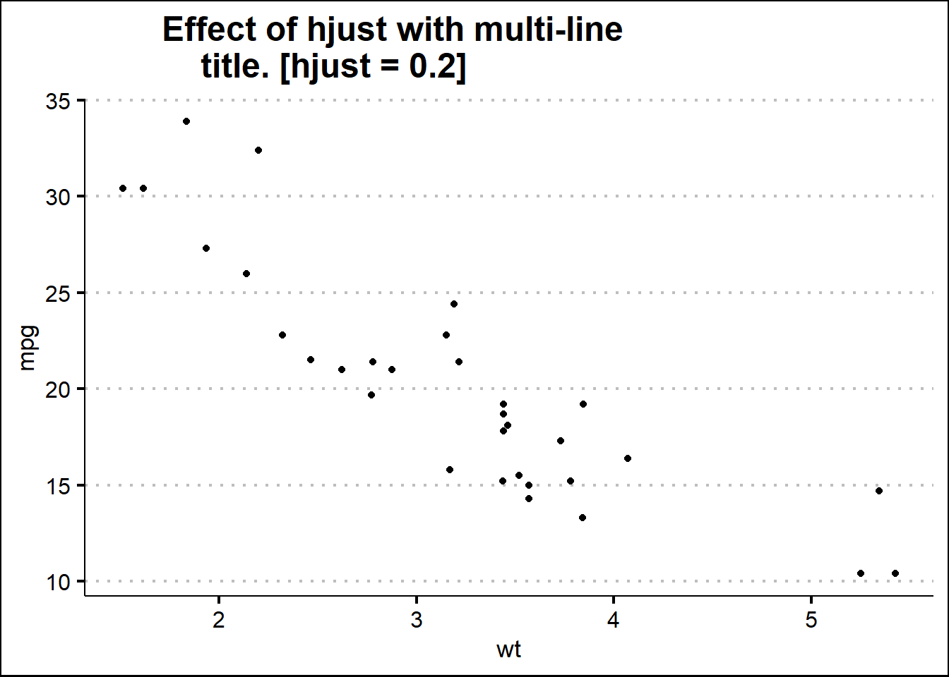
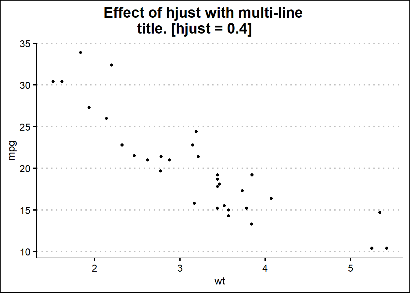
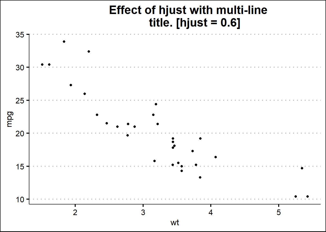
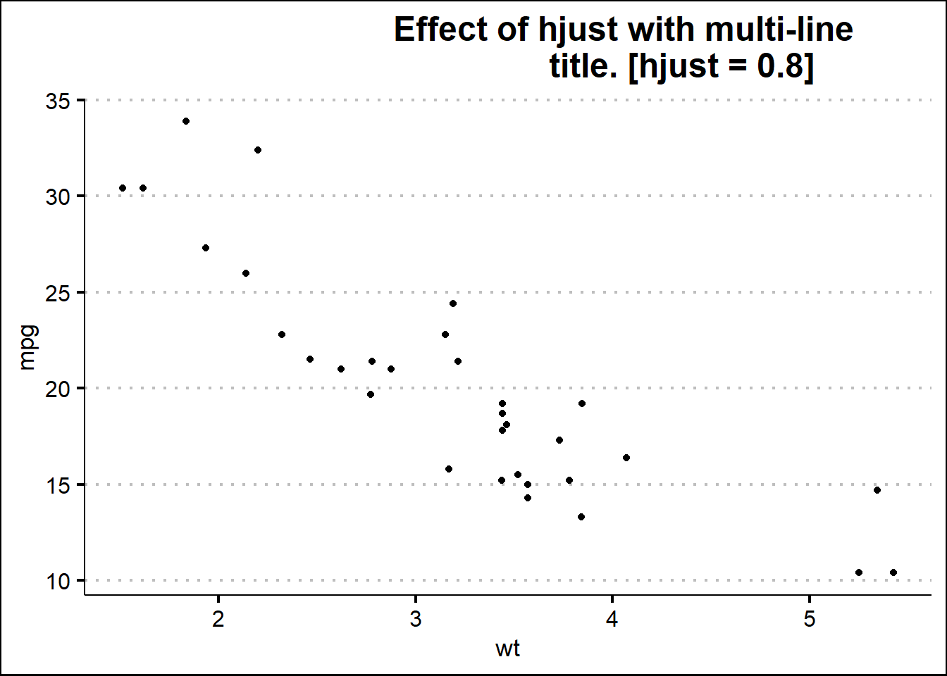
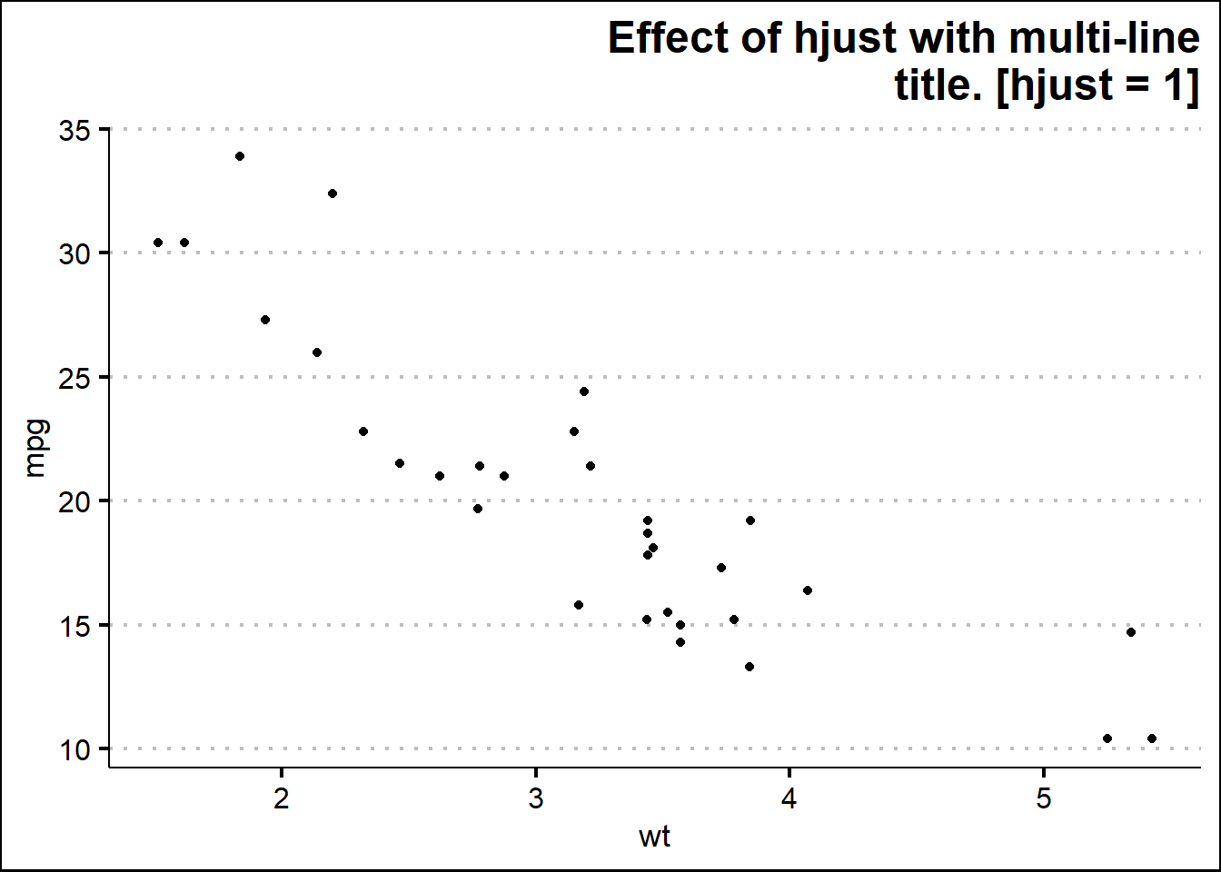
Systematically explore the effects of hjust when you have a multi-line title. Why doesn’t vjust do anything?

In ggplot2, the hjust and vjust parameters control the horizontal and vertical alignment of text, respectively. However, when you have a multi-line title, the vjust parameter doesn’t seem to have any noticeable effect. This is because ggplot2 calculates the vertical positioning of multi-line text differently from single-line text.

When you specify a multi-line title, ggplot2 automatically adjusts the vertical alignment of the text to center it within the available space. This behavior overrides the vjust parameter. Instead, ggplot2 focuses on aligning the entire multi-line text block within the plot title area.

On the other hand, the hjust parameter still has a significant impact when you have a multi-line title. It controls the horizontal alignment of the entire text block, shifting it left or right within the title area.

To systematically explore the effects of hjust with a multi-line title in ggplot2, here’s an example code snippet to illustrate this:

Code

# Create a basic plot with a multi-line title
p <- ggplot(mtcars, aes(x = wt, y = mpg)) +
  geom_point() +
  theme_clean(base_size = 16)

# Create a list of hjust values to explore
hjust_values <- seq(0, 1, by = 0.2)

for (i in hjust_values) {
  pp <- p + 
  theme(
    plot.title = element_text(hjust = i)) +
    labs(title = glue::glue("Effect of hjust with multi-line\ntitle. [hjust = {i}]"))
  
  print(pp)
}