Chapter 6

Maps

Author

Aditya Dahiya

Published

November 18, 2023

Note

This Chapter does not have Exercises. The code and examples below show map plotting in R with tidyverse and sf with examples from India.

Code

library(tidyverse)     # everything and ggplot2
library(sf)            # sf and shape files
library(ggthemes)      # for theme_map
library(ggspatial)     # map annotations
library(ggmap)         # to get base raster tiles for maps

# Reading in the shape file of the map of India
india_map <- read_sf(here::here("data", 
                                "india_map", 
                                "India_State_Boundary.shp")) |> 
  # tidy names of variables
  rename(state = State_Name) |> 
  # Renaming to official names. Official names taken from Government:
  # https://knowindia.india.gov.in/states-uts/
  mutate(state = case_when(
    state == "Andaman & Nicobar" ~ "Andaman and Nicobar Islands",
    state == "Daman and Diu and Dadra and Nagar Haveli" ~ "Dadra and Nagar Haveli and Daman & Diu",
    state == "Jammu and Kashmir" ~ "Jammu & Kashmir",
    state == "Telengana" ~ "Telangana",
    .default = state
  ))

# Add names of Union Territories
union_territories <- c(
  "Andaman and Nicobar Islands",
  "Chandigarh",
  "Dadra and Nagar Haveli and Daman & Diu",
  "Delhi",
  "Jammu & Kashmir",
  "Ladakh",
  "Lakshadweep",
  "Puducherry"
)

# Getting in a dataframe with map of State of Haryana in India
haryana_map <- read_sf(here::here("data",
                                  "haryana_map",
                                  "HARYANA_DISTRICT_BDY.shp")) |> 
  janitor::clean_names() |> 
  mutate(
    district = str_replace_all(district,
                               pattern = ">",
                               replacement = "A"),
    state = str_replace_all(state,
                            pattern = ">",
                            replacement = "A"),
    district = case_when(
      district == "FAR|DABAD" ~ "FARIDABAD",
      district == "J|ND" ~ "JIND",
      district == "PAN|PAT" ~ "PANIPAT",
      district == "SON|PAT" ~ "SONIPAT",
      .default = district
    ),
    district = snakecase::to_title_case(district)
      )

6.2 Simple features maps

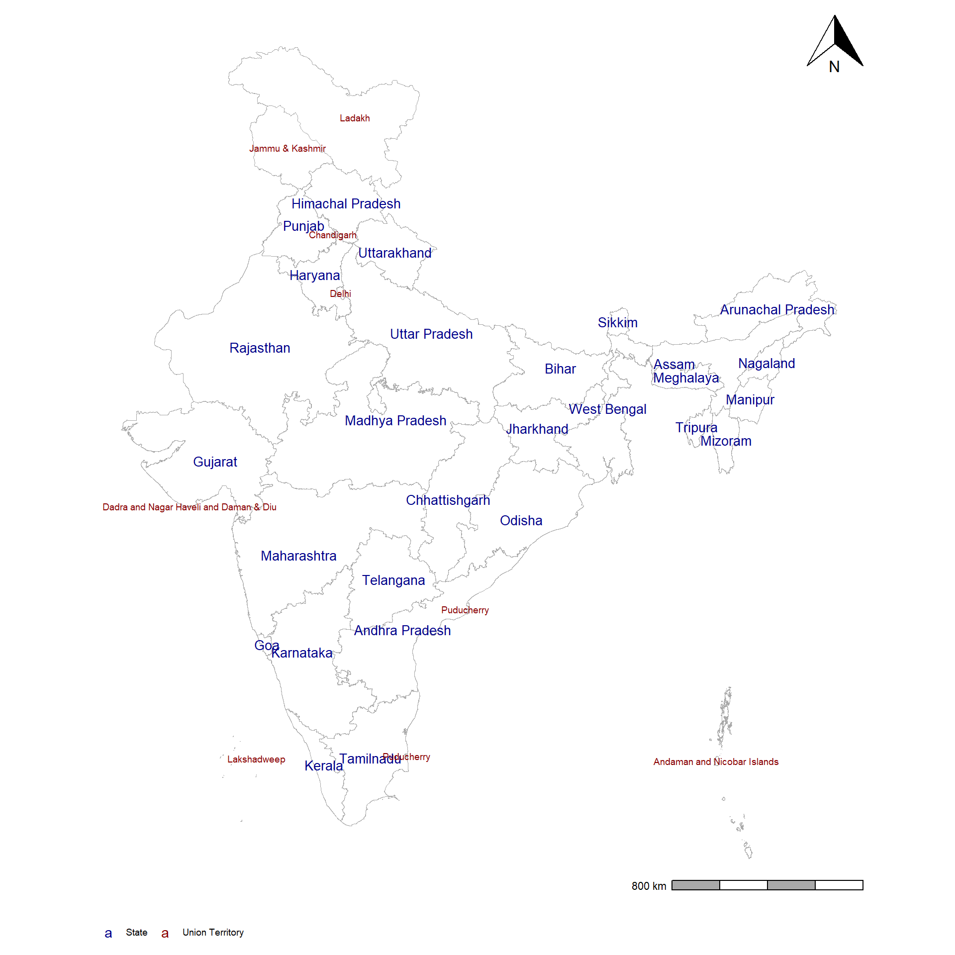
First, we download a shape file of India’s map (from here) and plot a map of India with latest state and Union Territory boundaries. The code below shows a simple example of ease of plotting with ggplot() and geom_sf() along with labeling official names of States and Union Territories.

Code

# Plotting the actual map
india_map |> 
  
  # A variable to use for different font colour for States vs. Union Territories
  mutate(type = if_else(state %in% union_territories,
                        "Union Territory",
                        "State")) |> 
  # Start Plot
  ggplot(aes(geometry = geometry,
             col = type)) + 
  geom_sf(col = "darkgrey", fill = "white") +
  geom_sf_text(aes(label = state,
                size = type)) +
  
  # Colour and Size Scales
  scale_color_manual(values = c("darkblue", "darkred")) +
  scale_size_discrete(range = c(3.5, 2.5)) +
  
  # Themes
  theme_map() +
  theme(legend.position = "bottom") +
  labs(col = NULL) +
  
  # Adding Scale and North Arrow
  annotation_scale(bar_cols = c("darkgrey", "white"),
                   location = "br") +
  annotation_north_arrow(location = "tr", 
                         which_north = "true") +
  guides(size = "none")

6.2.1 Layered maps and 6.2.2 Labelled maps

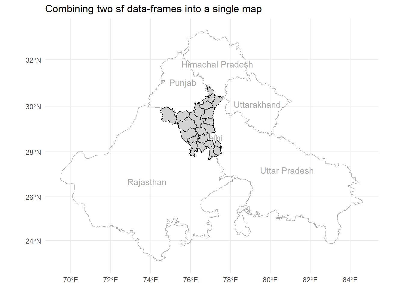
We can use data from multiple data-frames and add them as layers to a single map using ggplot2 as shown below: –

Code

# Names of Bordering states of Haryana
bordering_states = c("Punjab",
                     "Delhi",
                     "Himachal Pradesh",
                     "Rajasthan",
                     "Uttar Pradesh",
                     "Uttarakhand")

# Start plotting with India Map showing only bordering states
ggplot(data = india_map |> 
         filter(state %in% bordering_states),
       mapping = aes(geometry = geometry,
                     label = state)) +
  
  geom_sf(fill = "white",
          col = "darkgrey",
          alpha = 0.5) +
  geom_sf_text(col = "darkgrey") +
  
  # Map of Haryana with Districts
  geom_sf(data = haryana_map,
          fill = "lightgrey",
          col = "black") +
  
  # Labels and theme
  labs(x = NULL, y = NULL,
       title = "Combining two sf data-frames into a single map") +
  theme_minimal()

6.2.3 Adding other geoms

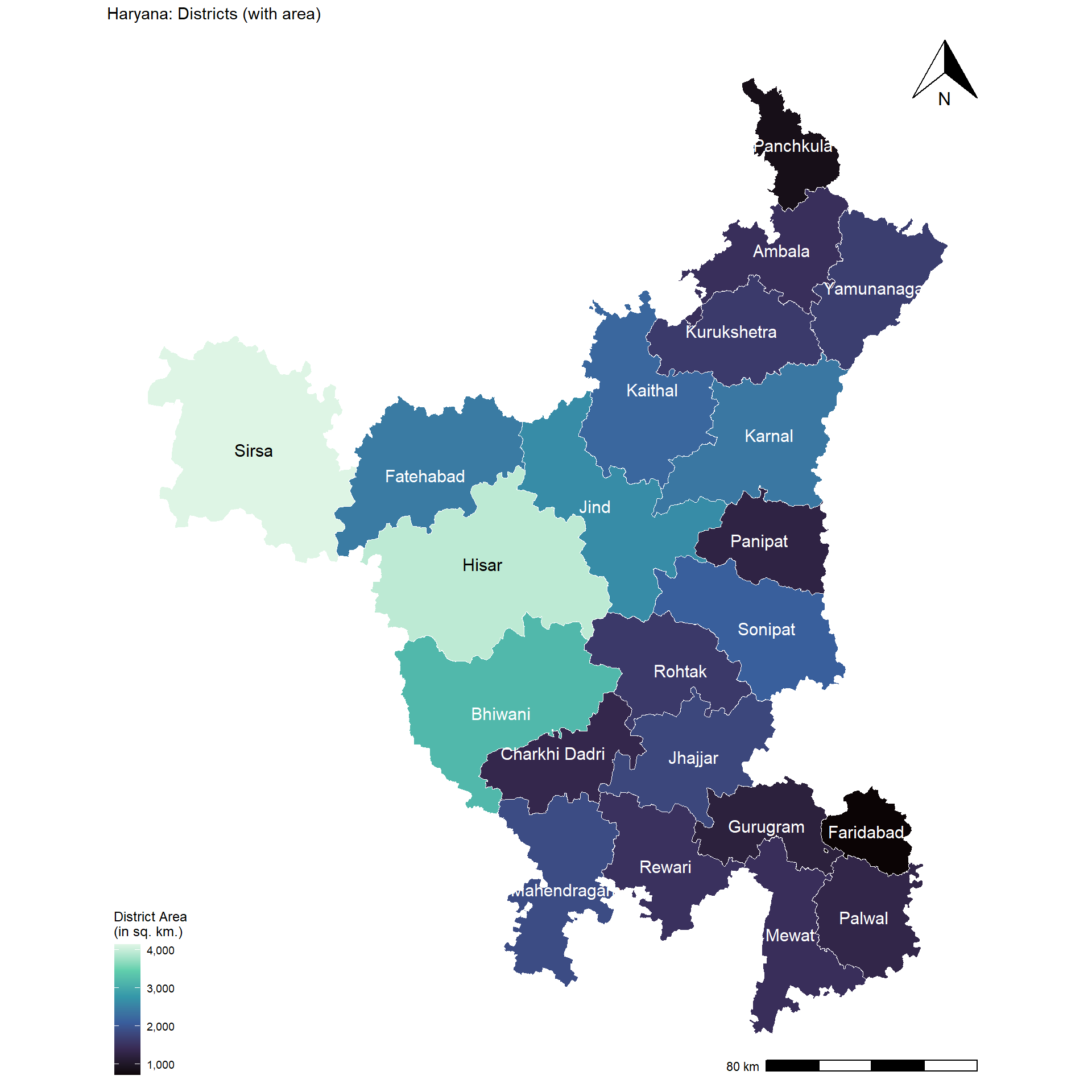
Plotting a specific state from i..e, Haryana, and its districts along with their area (in thousand sq. km.) using official data from Survey of India, and adding geoms from other metadata - area and length of district borders: –

Code

haryana_map |>
  select(-c(remarks, state_lgd, district_l)) |> 
  arrange(desc(shape_area)) |> 
  mutate(
    rank = row_number(),
    area = round(shape_area/1e9, 2),
    font_col = district %in% c("Hisar", "Sirsa")
  ) |> 
  
  ggplot(aes(geometry = geometry,
             label = paste0(district),
             fill = shape_area/1e6)) +
  geom_sf(col = "white") +
  geom_sf_text(aes(col = font_col),
               size = 4) +
  theme_map() +
  annotation_scale(location = "br") +
  annotation_north_arrow(location = "tr") +
  labs(fill = "District Area\n(in sq. km.)",
       title = "Haryana: Districts (with area)") +
  scale_fill_viridis_c(labels = scales::label_comma(),
                       option = "G") +
  scale_color_manual(values = c("white", "black")) +
  guides(col = "none")

Chloropleth with `tmap`

A package to create chloropleths very easily is the tmap package (Tennekes 2018) of R . However, is uses a very different syntax than ggplot2 . An interesting feature is the ability to plot interactive maps. However, since it is outside ggplot2 grammar and syntax, I do not use it here.

Code

library(tmap)
tm_hy <- haryana_map |> 
  mutate(area = shape_area/1e6)

t_hy <- tm_shape(tm_hy) +
  tm_polygons(col = "area",
              title = "District Area\n(in sq. km.)",
              border.col = "black",
              interactive = TRUE,
              style = "pretty")
t_hy
tmap_mode("view")
tmap_last()

tmap_mode("plot")

Adding `leaflet` maps to Chloropleths

Code

library(leaflet)

# Create a quantile of colours' palette to be used
pal_hy <- colorQuantile("Blues", 
                        domain = NULL,
                        n = 5)

# Create vector of text to display on pop-ups in leaflet map
p_popup <- paste0(haryana_map$district, 
                  " District.  Area: ", 
                  round(haryana_map$shape_area/1e6, 0),
                  " sq. km.")

# Create leaflet map
# Data set
haryana_map |> 
  
  # Transform polygons into CRS=4326 since leaflet only understand that
  st_transform(crs = 4326) |> 
  
  # Begin leaflet map
  leaflet() |> 
  
  # Add polygons from the geometry column of the data-set
  addPolygons(
    stroke = FALSE,                       # remove polygon borders
    fillColor = ~ pal_hy(shape_area/1e6), # set fill color with function
    fillOpacity = 0.6,                    # translucent to see background map
    smoothFactor = 0.5,                   # make it nicer
    popup = p_popup,                      # add popup
    group = "District Area"               # a Group label for leaflet options
  ) |> 
  
  # Add base map from leaflet; default is Open Street Maps
  addTiles() |>                           # Adding Base Map
  
  # Adding a legend
  addLegend(
    position = "bottomright",  # location
    pal = pal_hy,              # palette function
    values = ~shape_area/1e6,  # value to be passed to palette function
    title = "District Area (sq. km.)" # legend title
    ) |> 
  
  # Adding an option to view different base maps
  addLayersControl(
    baseGroups = c("OSM", "Carto"),
    overlayGroups = c("District Area")
  )

6.4 Working with `sf` data

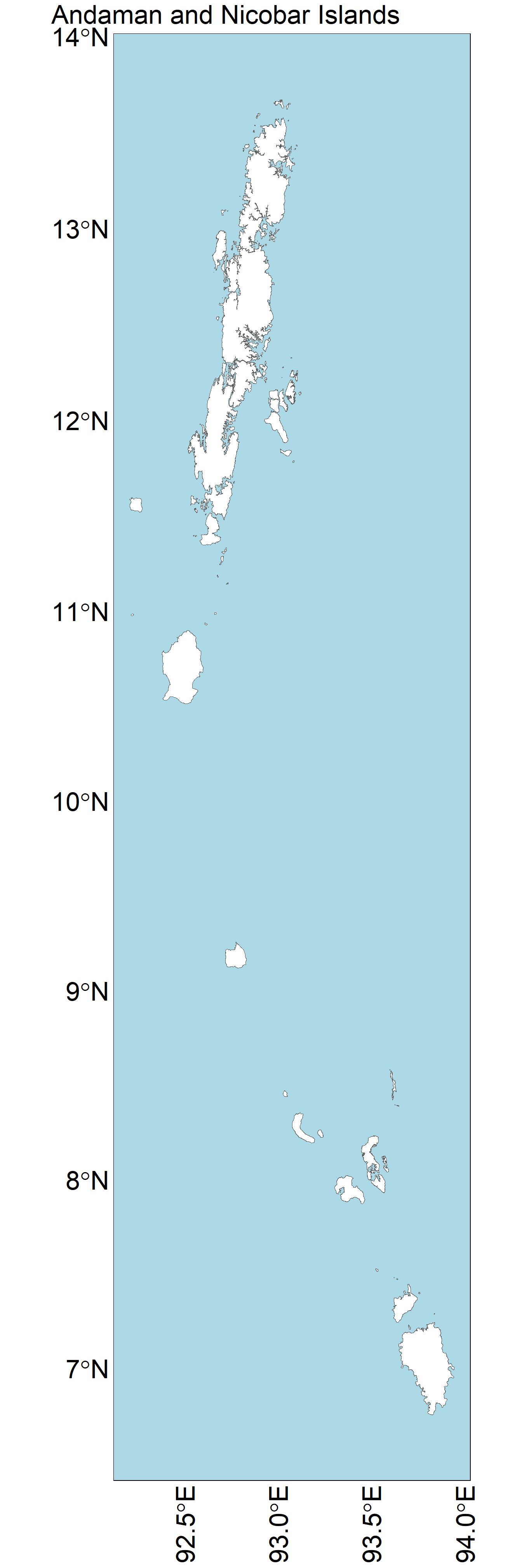
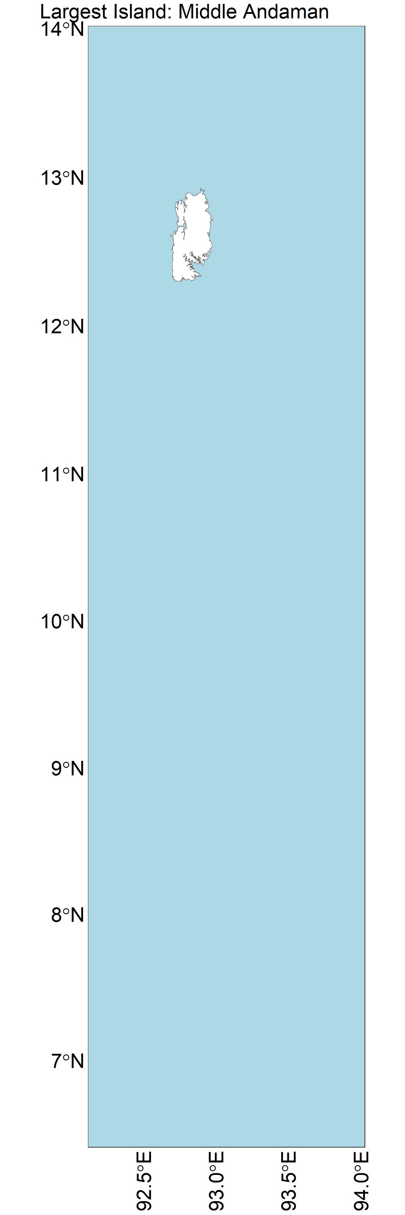
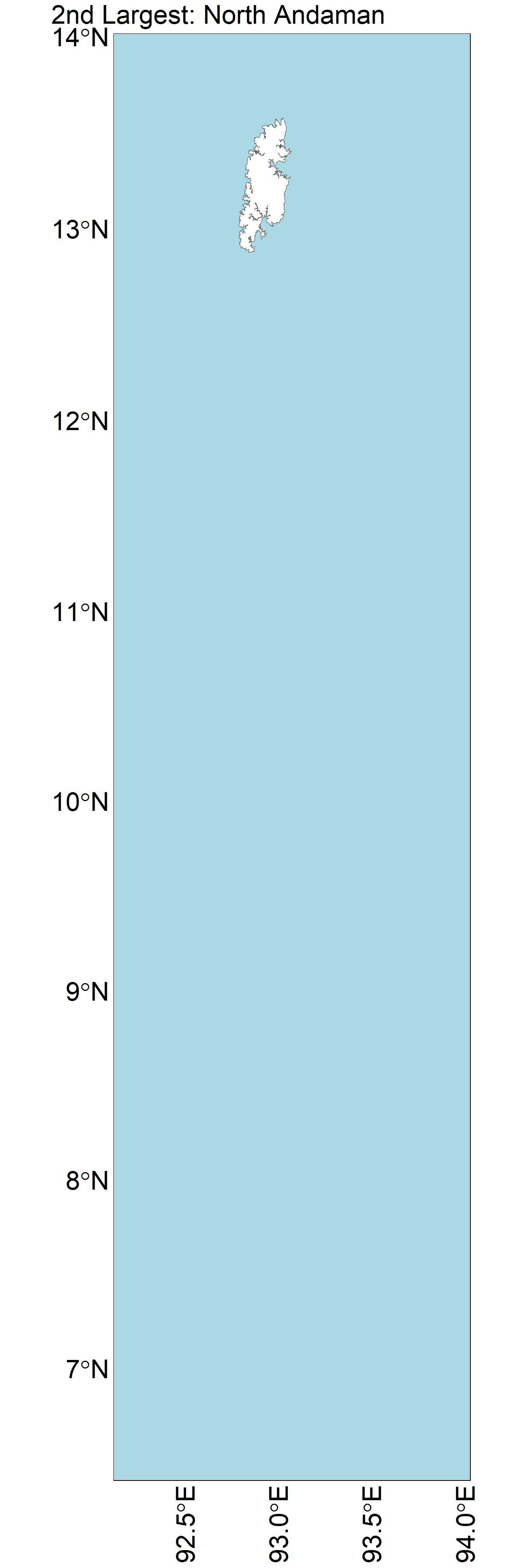
We can even drawn out different pieces of polygons, i.e. islands, enclaves or exclaves using sf data. The beauty of multi-polygon sf objects (i.e., geographic administrative units with more than one polygon, or, in simpler terms, groups of islands or non-contiguous areas) is that we can use st_cast(<object_name>, "POLYGON") to separate out each polygon (contiguous area unit) and order them by size using st_area() . We can pick out single polygons, even ordered by size, as we can see in Figure 1 (b) and Figure 1 (c) from an example using India’s Andaman and Nicobar Islands: –

Code

# Pull out the geometry of Andaman and Nicobar Islands as "ani"
ani <- india_map |> 
  filter(state == "Andaman and Nicobar Islands") |> 
  pull(geometry)

# Bounding Box of ani
lims <- st_bbox(ani)

# Create different polygon objects from a single multi-polygon 
ani_islands <- st_cast(ani, "POLYGON")

# Checking order: We see that islands are listed in decreasing order of size
# order(st_area(ani_islands), decreasing = TRUE)

# A common theme to use in all Island Maps
theme_islands <- theme_map() +
  theme(axis.text.x = element_text(angle = 90, 
                                   vjust = 0.5,
                                   size = 25),
        axis.text.y = element_text(vjust = 0.5,
                                   size = 25),
        plot.title.position = "plot",
        panel.background = element_rect(fill = "lightblue"),
        plot.title = element_text(size = 25))

# Drawing the complete Andaman and Nicobar Islands
india_map |> 
  filter(state == "Andaman and Nicobar Islands") |> 
  ggplot() +
  geom_sf(fill = "white") +
  labs(title = "Andaman and Nicobar Islands") +
  scale_x_continuous(limits = c(lims["xmin"], lims["xmax"])) +
  scale_y_continuous(limits = c(lims["ymin"], lims["ymax"])) +
  theme_islands

# Drawing the largest of the Andaman and Nicobar Islands
ggplot(ani_islands[1]) +
  geom_sf(fill = "white") +
  labs(title = "Largest Island: Middle Andaman") +
  scale_x_continuous(limits = c(lims["xmin"], lims["xmax"])) +
  scale_y_continuous(limits = c(lims["ymin"], lims["ymax"])) +
  theme_islands

# Drawing the second largest of the Andaman and Nicobar Islands
ggplot(ani_islands[2]) +
  geom_sf(fill = "white") +
  labs(title = "2nd Largest: North Andaman") +
  scale_x_continuous(limits = c(lims["xmin"], lims["xmax"])) +
  scale_y_continuous(limits = c(lims["ymin"], lims["ymax"])) +
  theme_islands

6.6 Data Sources

To obtain shapefiles for various states and administrative units of India from the Survey of India, you can visit their official website at https://onlinemaps.surveyofindia.gov.in/Digital_Product_Show.aspx. The Survey of India provides digital products, including shapefiles, and many of them are available free of cost.

Another valuable source for obtaining administrative boundary shapefiles is https://gadm.org/. GADM (Global Administrative Areas) offers global administrative maps and data, including those for India. Both Survey of India and GADM are reputable platforms that cater to the geographical data needs of researchers, analysts, and the public, making it convenient to access accurate and up-to-date spatial information.

References

Tennekes, Martijn. 2018. “Tmap: Thematic Maps in r” 84. https://doi.org/10.18637/jss.v084.i06.

6.2 Simple features maps

6.2.1 Layered maps and 6.2.2 Labelled maps

6.2.3 Adding other geoms

Chloropleth with tmap

Adding leaflet maps to Chloropleths

6.4 Working with sf data

6.6 Data Sources

References

Chloropleth with `tmap`

Adding `leaflet` maps to Chloropleths

6.4 Working with `sf` data